Video made using the PIC/FLIP solver we'll implement in this tutorial!

Physics-Based Simulation & Animation of Fluids

By Chand T. John, Ph.D.

Do you ever wonder how special effects using fluids like water are animated for movies? In this tutorial, we'll show you how to simulate fluids using the popular Particle-in-Cell / Fluid-Implicit-Particle (PIC/FLIP) method. In this tutorial, we will:

• write all the code, from scratch, for a physics-based fluid simulation,
• derive our code implementation from a widely used mathematical model of fluid physics,
• install minimal, widely available free software,
• not skip any steps, and
• follow professional code style and testing practices.

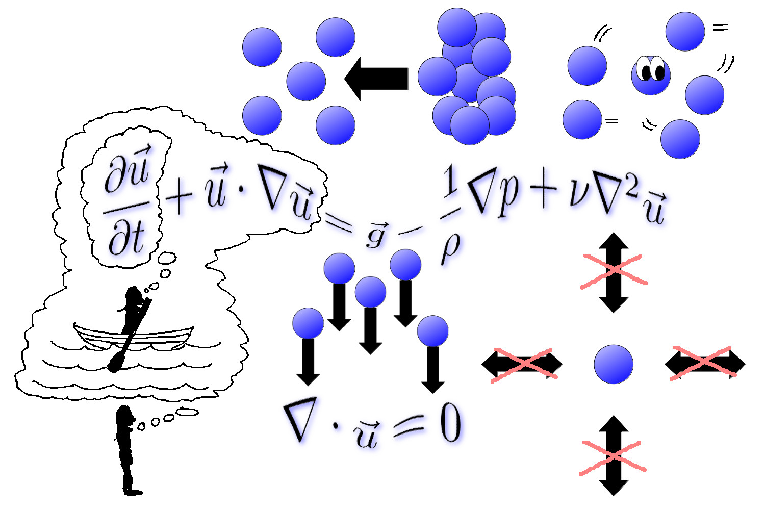
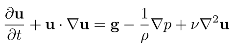
The mathematical model of fluid physics driving this tutorial are the Navier-Stokes equations, which we'll personify with this image, without explanation, for now. We'll dive into the details of these equations when introducing fluid mechanics below.

Acknowledgments

This tutorial expands on the fluid simulation portion of the excellent SIGGRAPH course on physics-based animation created by Dr. Adam Bargteil and Dr. Tamar Shinar. This tutorial also references the excellent educational materials on fluid simulation put together by Dr. Robert Bridson and Dr. Matthias Müller-Fischer as well as Dr. Bridson's book on fluid simulation. These resources are tremendously useful for making physics-based simulation and animation accessible to a wide audience and I merely hope to add some details and illustrations on top of these awesome contributions by others. We will cite all of these materials frequently throughout this tutorial! I highly recommend going through these materials if you are at all curious about physics-based simulation for computer graphics.

Background

This tutorial is designed assuming a year or two of experience in or exposure to:

• Computer programming in C++
• Using a command-line terminal on a computer running Linux, e.g., the Ubuntu operating system
• Newtonian mechanics, e.g., F = ma, momentum, position, velocity, acceleration
• Calculus: differential, integral, and vector calculus

Some exposure to computer graphics helps but is certainly not required. If you're a second- or third-year computer science college student, you have more than enough background! If you haven't gone to college, haven't studied computer science, don't remember much math or physics, or this list just feels overwhelming in general, that's okay! Feel free to follow along and look up and/or skip lots of things! You don't have to understand everything, by any means, to gain something from this tutorial. Other than access to a computer (yes, this can be a challenge) and at least an occasional Internet connection, everything else this tutorial requires is freely available!

What to Install

This tutorial will use the C++ programming language. We will use the Open Graphics Library (OpenGL) and the associated OpenGL Utility Toolkit (GLUT) to display graphics on the computer screen. This is freely available software widely used for displaying graphics on computer screens.

From this point onward, I'll assume you're using a computer running Ubuntu 16.04 or 18.04. I'll also assume your computer account has permission to install new software on that computer, or if not, that someone else can do it for you. If you're running another operating system, such as Windows or macOS, you should be able to follow along but with some small changes to commands and the code.

Open a Terminal (CTRL+ALT+T on Ubuntu). Type this command and press Enter:

g++ --version

You should see some text showing the version of g++, the program we'll use to compile our code, that is installed on your computer. If not, look up how to install it. For our purposes, which version of the compiler you install should matter much.

Next, in a Terminal (the same one as before is fine!), type this command and then press Enter to run it:

sudo apt install freeglut3-dev

If you're asked to, enter your password and press Enter. Once the computer finishes installing OpenGL and GLUT, figure out where it was installed. I found this out by typing something like ls /usr/lib/x86_64-linux-gnu/libgl* and pressing the [TAB] key twice, causing the Terminal to list a whole bunch of files with names starting with libglsomething including libglut.something. So, my OpenGL and GLUT libraries were installed in /usr/lib/x86_64-linux-gnu/. Feel free to search online for how to find where OpenGL and GLUT were installed on your computer if you're not sure.

This is not required but I highly recommend installing clang-format, a program used by many software developers in industry to format their code in a consistent style. We'll use this program to format our code in Google's style. To install it, run this command in a Terminal and press Enter:

sudo apt install clang-format-10

It's okay to use another version of this program; I just happen to be using version 10 at the moment.

Now, create a directory (folder) somewhere on your computer where you want to store all the code you write as part of this tutorial. You can and will make multiple subdirectories in there as the tutorial proceeds, but it's good to have one parent directory that holds everything. cd to that parent directory in a Terminal window. Then type this command and press Enter:

clang-format-10 -style=Google -dump-config > .clang-format

This creates a "hidden" file (meaning you can see it by running the ls -a command, but not the plain ls command) in this directory that contains your default settings consistent with the Google style for the clang-format program. Here is my .clang-format file. If for some reason you want to keep your code in multiple disparate places on your computer, you can just re-run this command in each of those directories.

Why Physics?

Why do we use physics and math to derive code that simulates a fluid? It's actually quite hard to animate fluid motion in a way that looks believable enough for movie viewers. It's also become more feasible as computers have become more powerful, to simulate accurate physics rather than try to fake it.

To make physics into something we can compute, though, we must use math. In physics, the terms "mechanics" or "dynamics" typically refer to the mathematical relationships between motion (kinematics) and the forces (kinetics) that generate that motion. You'll often hear the terms "fluid mechanics" and "fluid dynamics" used interchangeably. The whole point is to determine how forces lead to motion, mathematically, so that a computer can do that math and simulate that motion for animation. Fluid simulation is also very important in scientific applications, including weather prediction.

Viewing Geometry Using OpenGL

OpenGL is a general framework that allows us to do graphics programming. To use it to display geometry effectively, we need to set up some initial working code and understand a bit about how OpenGL code manages what we see on the screen.

Hello, Sphere!

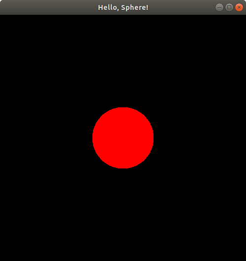
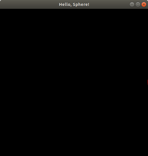
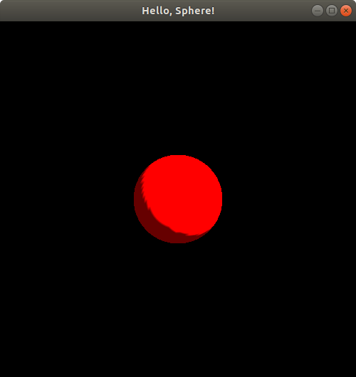
Our first program will be a single file containing code in the C++ programming language. When we run this program, if everything is working, a window will pop up on the computer screen displaying a single, red, boring sphere. It's so boring, in fact, that it won't even look three-dimensional: it'll just look like a filled-in red circle.

Make a directory called basic inside the directory that'll house all your code for this tutorial. Okay, you can put this directory anywhere, but this will just make it less work for you to run clang-format on your code and keep it organized the same way as this tutorial's code. In that directory, create a file called HelloSphere.cpp. You can copy the code from my HelloSphere.cpp file and save it. Or you can just download the file by clicking on this link and then clicking the "Raw" button on that page. I put a lot of comments in the file explaining what the code does. If you want to learn more details about how OpenGL and GLUT work, you can find plenty of documentation via online search.

In a Terminal, cd to the directory containing this HelloSphere.cpp file. Then run this command:

clang-format-10 -style=file -i HelloSphere.cpp

Congratulations! Your C++ code is now formatted according to Google's standards! Well, at least it's formatted to the standards a computer can follow automatically. Now, let's compile your code with this command:

g++ HelloSphere.cpp -o HelloSphere -L/usr/lib/x86_64-linux-gnu/ -lGL -lglut -lGLU

If it compiled with no errors or warnings, let's run the program! Run it with this command:

./HelloSphere

You should see a window pop up on your screen that looks something like this:

You can close the window to stop the program.

Here are a couple sources that I think illustrate nicely how to create simple OpenGL programs from scratch:

• StackOverflow example on displaying a sphere in OpenGL
• First tutorial from the OpenGL Step by Step series

It's exciting to get our first program working. But the geometry I claimed was 3D just looks like a boring red disc (filled-in circle). How can we make it look 3D?

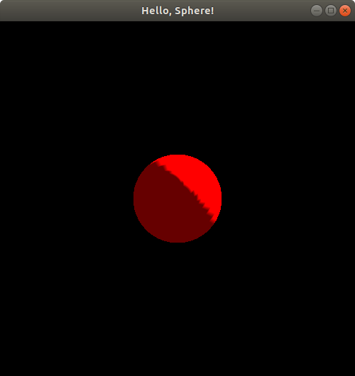
Hello, Shaded Sphere!

The 3D nature of shapes becomes more apparent when we add shading to our scene. In OpenGL, this is done by modeling the effects of light on the color of each vertex of any shape, assuming some material properties of the shape. By turning on a light, we can make our sphere "look" three-dimensional. In the same directory as the previous program (just for convenience, e.g., access to the same .clang-format file), create a new file called HelloSphereShaded.cpp. Here is my version, which you can copy or download: HelloSphereShaded.cpp.

Compile the program:

g++ HelloSphereShaded.cpp -o HelloSphereShaded -L/usr/lib/x86_64-linux-gnu/ -lGL -lglut -lGLU

Run it:

./HelloSphereShaded

View the result:

And there you have it! Now there's some shading, revealing the 3D shape of our sphere!

To clarify exactly how the 3D coordinates of our shapes map to the 2D locations of shapes we see on the computer screen, let's do some experiments.

Positioning the Sphere

Make a new program called PositionSphere.cpp in the same directory (for convenience, you could put it in another directory if you really want). Here's my code: PositionSphere.cpp.

Compile this program:

g++ PositionSphere.cpp -o PositionSphere -L/usr/lib/x86_64-linux-gnu/ -lGL -lglut -lGLU

Run it:

./PositionSphere

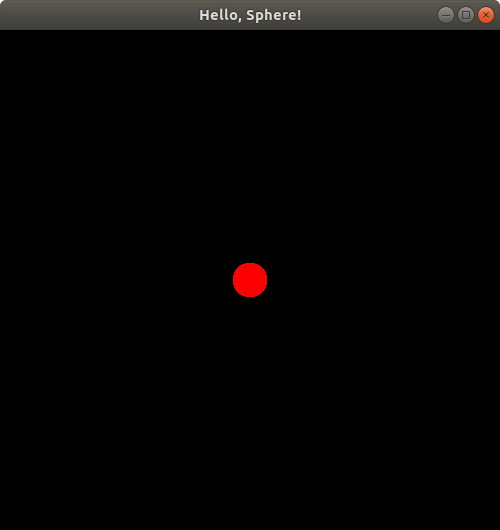
The window that pops up should look exactly the same as before! Now let's change the call to putSphereCenteredAt to putSphereCenteredAt(1.0, 0.0, 0.0); and then compile and run the program using the same commands as before. Here's the result:

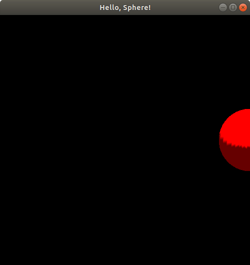
Hmm. It looks like the sphere is halfway out of our viewing window! Let's push the boundaries a bit further by changing that function call to putSphereCenteredAt(1.2, 0.0, 0.0);, compiling, and running again. Here's the result:

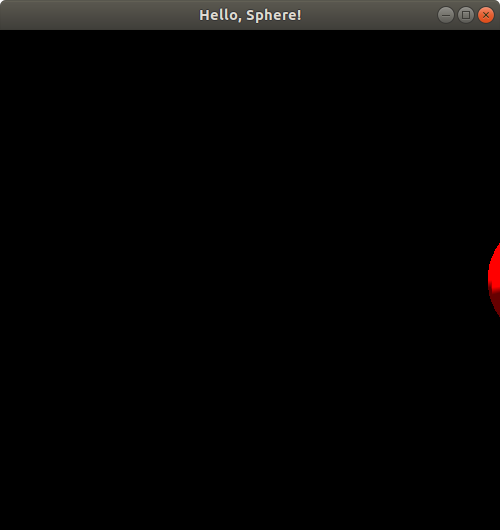
The sphere is almost gone--just a little sliver left! Now, you might notice from the code above that the radius of this sphere is 0.25. We have just moved the sphere to the right by 1.2. If the viewing window is showing us x-coordinate values ranging up to x = 1, and if the positive x-axis direction points to the right of our window, then we would expect the sphere to disappear completely when we shift it to the right (positive x direction) by 1.25 or more. Let's try putSphereCenteredAt(1.245, 0.0, 0.0);:

Sure enough, we only see a tiny sliver of the sphere remaining in our viewing window! If you're having trouble seeing it, it's just a few red pixels on the right middle end of the image above. Finally, let's try putSphereCenteredAt(1.25, 0.0, 0.0);. Sure enough, the resulting image, which I won't bother to show you here due to its extremely boring pitch black appearance, displays absolutely no part of the sphere. So, it seems like a reasonable guess, that perhaps our viewing window extends up to x = 1 on the right side.

Similar experiments will reveal that the left end of our viewing window extends to x = -1, the top end goes to y = 1, and the bottom goes to y = -1. To verify this yourself, try putting 1.245 or -1.245 into the x or y coordinates of the putSphereCenteredAt function call one at a time and observe where the little sliver of the sphere appears.

The z-coordinate is a bit odd in comparison. Let's try the same experiment, first with putSphereCenteredAt(0.0, 0.0, 0.75);:

If you compare this image to the original one from the first time we ran this program with no translation, or equivalently, the picture we got when we ran HelloSphereShaded.cpp, you may notice that the spheres look exactly the same size; the only difference between them seems to be the lighting and shading. This may seem a bit strange since the z-axis is presumably oriented somehow toward/away from us, i.e., perpendicular to the computer screen (since the x- and y-axes are both parallel to the computer screen), yet, unlike real life, bringing the sphere closer to us doesn't seem to be changing its size!

Let's continue experimenting. Let's now move the sphere to putSphereCenteredAt(0.0, 0.0, 1.0);. If you run this, you'll notice a totally blank, black window again! What happened to the sphere? Why did it disappear? If z is clamped to [-1, 1] like x and y are, should we still see half of the sphere in our viewing window when we move it to be centered at z = 1?

Let's make one other change to the code, temporarily. Let's comment out these two lines in the drawBackground() function:

  // glEnable(GL_CULL_FACE);
  // glCullFace(GL_BACK);

Then, try running the program:

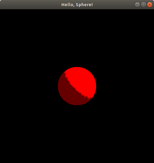
Now, we seem to see the sphere again--the lighting looks different than what we just saw earlier. Let's not analyze the lighting too much and let's keep moving the sphere further along the z-axis. Let's move it now to putSphereCenteredAt(0.0, 0.0, 1.24);:

Hmm. Looks like the sphere is starting to disappear! Let's try putSphereCenteredAt(0.0, 0.0, 1.2499);:

Just a tiny dot of the sphere left in our viewing window! Change the z-coordinate to 1.25 to verify that the sphere does indeed completely disappear from the viewing window at that location. This suggests pretty strongly that the z-coordinate does indeed extend up to z = 1 on the positive side of the z-axis (since the sphere has radius 0.25, so if it's centered at z = 1.25, the points on its surface will have z values that go as low as 1.25 - 0.25 = 1, which we can't see, and if it's centered at z = 1.2499, its points will go as low as z = 1.2499 - 0.25 = 0.9999, of which we do see a tiny bit). But is the positive z direction pointing toward us, or away from us?

If you do the exact same experiments but with negative z values (and now you can uncomment those lines of code that mentioned something about culling), you'll notice the exact same pattern. When the sphere is centered at (0.0, 0.0, -1.0), it appears to have exactly the same size as it did at z = 0.75 and at z = 0, but with just a bit of a change in its lighting and shading:

If you continue the experiment to move the sphere's center to (0.0, 0.0, -1.2499), you'll notice an identical image to when we put the sphere center at (0.0, 0.0, 1.2499), i.e., just a tiny dot in the middle of the screen is visible, and if you move the sphere center to (0.0, 0.0, -1.25), you'll see a totally blank black screen like you did when you moved the sphere center to (0.0, 0.0, 1.25). So, it appears that the negative z-coordinate also extends up to z = -1.

How OpenGL Maps from 3D to 2D

It still seems bizarre that with all this experimenting, we can't tell whether z increases toward us, or decreases toward us! But at least we did discover that we seem to be able to view any points that are within (-1, 1)³ ⊂ R³, i.e., a box where -1 < x, y, z < 1. This is called OpenGL's default viewing frustum. We also figured out that x increases to the right and y increases upward. Based on this, it might be a reasonable guess that z by the right-hand rule increases toward us. But how can we know for sure?

Instead of experimenting indefinitely, let's now get a more detailed understanding of exactly what OpenGL does to go from what appears to be 3D geometry, to a 2D image on our two-dimensional computer screen.

The glutSolidSphere function always generates a set of triangles that approximate the surface of a sphere that is centered at (0, 0, 0). To "move" a sphere to be centered at a location other than (0, 0, 0), we must adjust the coordinates of the vertices of the triangles approximating the sphere to be located in appropriate places such that the resulting sphere would be centered at the desired location. To handle this shifting, or translation, of the coordinates, our code calls the glTranslated function. But notice some other code around that function call: there is some pushing and popping of a matrix, and something called GL_MODELVIEW. What is all that?

OpenGL actually transforms the coordinates of any points it draws in the following way. Let (x, y, z) be an arbitrary point, e.g., a vertex on one of the triangles making up the sphere created by a call to glutSolidSphere. OpenGL represents each point in homogenous coordinates, so the point is represented with the coordinates p = (x, y, z, 1). These original coordinates for the point p are said to be in the object coordinate system or local coordinate system. The terms "local" and "object" here are referring to coordinate system whose origin is at the center of the sphere itself, regardless of where we're trying to center it. So, this is the coordinate system that is "local" to the "object," i.e., the sphere we want to draw. OpenGL represents this 4D point as a column vector (4x1 matrix) and then left-multiplies it by a 4x4 model matrix. The resulting 4x1 column vector represents the same point in the world coordinate system of OpenGL. This is the default, universal coordinate system OpenGL uses. All other coordinate systems are defined relative to this coordinate system. Note that this coordinate system isn't explicitly defined anywhere; a universal coordinate system just exists theoretically, and the only way for us to "see" it is to define at least one other coordinate system from which to view the universal/world coordinate system. Next, OpenGL left-multiplies that world-coordinate-system 4x1 column vector by a 4x4 view matrix. The resulting 4x1 column vector represents the point p's coordinates in what we call the view coordinate system. Next, OpenGL left-multiplies this 4x1 vector by yet another 4x4 matrix called the projection matrix, yielding a 4x1 vector of coordinates for the point p in the clip coordinate system. At this point, OpenGL "clips" or removes all points that lie outside of the viewing frustum. In this case, we're using OpenGL's default viewing frustum where the x, y, and z coordinates must lie within (-1, 1). After clipping, OpenGL normalizes the coordinates of all remaining points so that x, y, and z lie within (-1, 1). By default, the clip coordinates are already in that range as we just said, but OpenGL does allow you to change the clip coordinates to be in a different range. But when OpenGL normalizes the clip coordinates into the normalized device coordinate (NDC) system, the coordinates must all lie within (-1, 1) regardless of what range the clip coordinates cover. Finally, the NDC coordinates are transformed so that -1 < x_ndc < 1 covers 0 < x_window < w, where w is the width of the viewing window specified in the code above, -1 < y_ndc < 1 covers 0 < y_window < h, where h is the height of the viewing window, and -1 < z_ndc < 1 covers 0 < z_window < 1. It is possible to change these ranges in OpenGL, but what we described here is the default behavior of OpenGL.

Let's denote the model matrix by M_model, the view matrix by M_view, and the projection matrix by M_proj. Then the clip coordinates, p_clip, of the point p in object coordinates is p_clip = M_proj · M_view · M_model · p. Let w = h = 500 pixels, as specified in our code above for the window size.

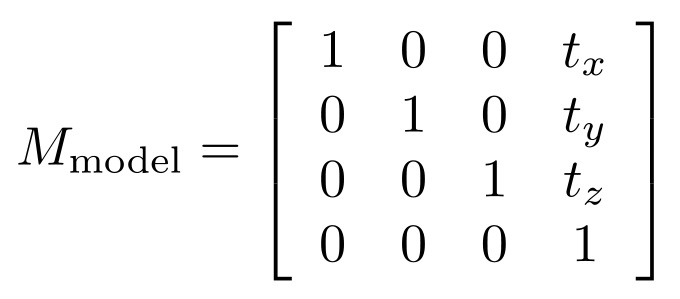
In our HelloShadedSphere.cpp and original PositionSphere.cpp programs, when we left the sphere centered at the origin of the world coordinate system, our model matrix, M_model, was the 4x4 identity matrix. Later when we started translating the sphere away from being centered at the origin, that translation amount, (t_x, t_y, t_z) (e.g., once we did t_x = t_y = 0 and t_z = 1.2499), was included in the model matrix. That is:

The view matrix is what represents the position and orientaton of the "camera" of OpenGL. By default, this is the identity matrix. This effectively makes us view all the objects in our OpenGL scene, by default, by having our camera eye located at (0, 0, +∞), while looking in the negative z direction. You'll see other sources saying the camera eye is effectively at the origin, (0, 0, 0), but the projection we describe below actually makes the concept of the eye being anywhere near the scene seem nonsensical. So, by default,

,

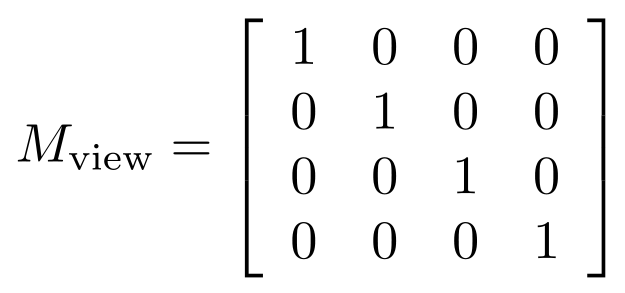but if you look at our code above, you'll notice that the model matrix and any view matrix are all combined into a single stack of matrices OpenGL calls the GL_MODELVIEW matrix mode. So, OpenGL actually combines, at any point in the code, model and view matrices into a single matrix that gets applied to all object-space vertex coordinates to obtain view coordinates. In our case,

.

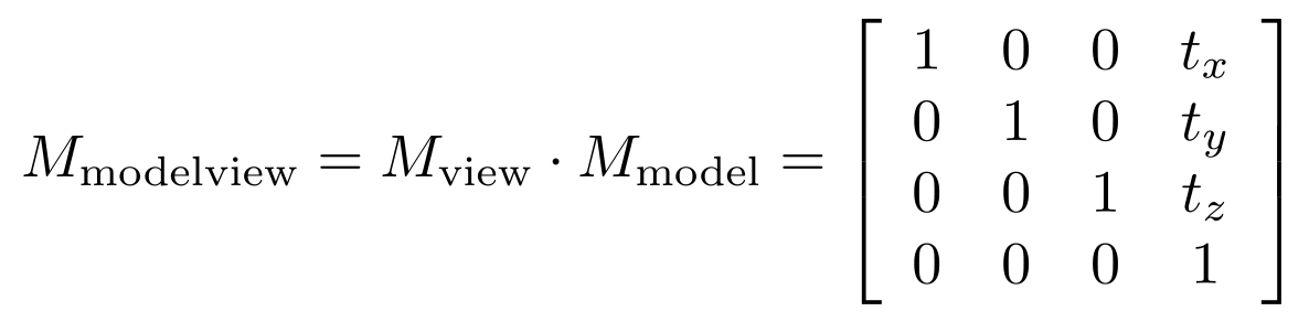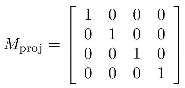
By default, in OpenGL, M_proj is the 4x4 identity matrix, which represents what is called an orthographic projection: it's like having a camera located infinitely far away from the origin, which lacks any notion of perspective; everything looks just as close to us as everything else since everything is, basically, infinitely far away from us. It's kind of like how we can't tell which stars in the sky are closer or farther away from us just by looking at them, even though we can judge how close a basketball might be to us if it's 1 meter vs. 10 meters away. With the default orthographic projection in OpenGL, it's like everything is a star that's infinitely far away. OpenGL applies the projection matrix typically on another matrix stack called GL_PROJECTION, which is not mentioned in our code since we just used the default projection matrix. If we wanted to change the camera's behavior, we could do so explicitly on the GL_PROJECTION matrix stack in our code. So:

Combining all of this, we see that p_clip = M_proj · M_view · M_model · p = (x + t_x, y + t_y, z + t_z), i.e., the result of the projection and modelview matrices, together, is just to translate all object-space coordinates of all points by (t_x, t_y, t_z). After applying all of these transformations, OpenGL will clip any points that are outside of the viewing frustum, like we saw earlier in all the examples where parts of the sphere were cut off from appearing in the viewing window.

Since our clip coordinates are already normalized by default, p_clip also represents the normalized device coordinates (NDC) of all points: p_ndc = p_clip. Finally, the NDC coordinates are transformed to window coordinates by scaling and shifting the NDC values to get the x-coordinates to be within 0 to w, the y-coordinates to be within 0 to h, and the z-coordinates to be within 0 to 1. This is accomplished by setting x_window = (w/2)(x_ndc + 1) pixels, y_window = (h/2)(y_ndc + 1) pixels, and z_window = (1/2)(z_ndc + 1). You can verify that x_ndc = -1 gets mapped by this transformation to x_window = 0 and x_ndc = 1 gets mapped to x_window = w = 500, so this is how the 3D object coordinates end up getting mapped to 3D window coordinates.

Finally, what we see on our 2D screen is the result of taking the 3D window coordinates and doing a depth test, as we asked OpenGL to do with in our code with the function call glEnable(GL_DEPTH_TEST);. So, this is how OpenGL makes sure whatever we see on our 2D screen is whatever is closest to us in the 3D scene we defined, much like a real-life camera's 2D image displays what the camera can see in a 3D real-world scene.

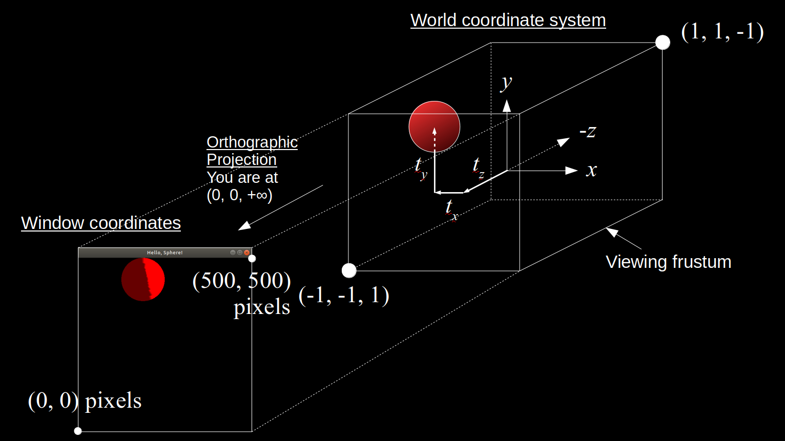
All of these coordinate system shenanigans were to help us understand exactly what we see on the screen, and how what we see in pixels maps to the original 3D coordinates of the objects we constructed. This insight will come in handy as we start moving objects around on the screen during animations of physics-based simulations! Here is a diagram summarizing the overall default transformation from world coordinates to window coordinates in OpenGL:

For more details and insights on how OpenGL handles coordinate transformations read these sources:

• Official OpenGL documentation on viewing and transformations
• LearnOpenGL article on coordinate transformations
• Detailed description and derivation of OpenGL transformations
• Stack Overflow post and answer on orthographic projections
• OpenGL matrix modes and order of projection and modelview matrix multiplications

Now that we understand, in detail, how our 3D world scene maps to our 2D window, we can proceed to implementing animations of physics-based simulations using OpenGL. Note that with our current setup, the 2D location of the center of a sphere in the window on our computer screen accurately shows the location of the sphere's center in the xy-plane in the world coordinate system, since the orthographic projection does not distort this 2D location in any way.

A Massless, Sizeless Particle

We'll go through a few steps to describe each physics-based simulation in each tutorial:

1. Describe a mathematical model of the physical system we want to simulate.
2. Design and implement that mathematical model in a computer program.
3. Run the program and view the results.

Mathematical Model of a Massless, Sizeless Particle

Like Dr. Adam Bargteil and Dr. Tamar Shinar's course on physics-based animation from SIGGRAPH 2018 and 2019, we begin by considering a very simple object to simulate: a theoretical particle that is infinitely small and has no mass. You can't see it. You can't feel it. It's almost as if it isn't there at all. Oh, but it is there, if we define it to be: an infinitely small dot, moving around in space, or sitting still in space, that defies all of our senses. In a nutshell, a particle, p, is nothing but a vector function x_p(t) of time t representing the position of the particle at any given time. We can think of a simulation of a massless, sizeless particle as just us sitting there staring at a sequence of (x, y, z) coordinates changing over a period of time, scrolling by on our computer screens before our eyes. Here is a more formal definition.

Definition. Let T be a closed interval in the set of real numbers, R. Each element of T is called a time or instant of time. A particle, p, is a function x_p: T → R³ that assigns to every time t ∈ T a position, x_p(t) = (x(t), y(t), z(t)), in 3D space, where x, y, z: T → R are functions representing the coordinates in 3D space of the particle p at each time, t.

We'll refrain from formally defining what a simulation of a massless, sizeless particle is (even though we will basically do it here, but note the details of this "definition" will change as we deal with different systems in this tutorial), but you can think of it simply as a discrete sampling of the position function x_p(t) at specific instants in time. That is, if we pick a strictly increasing sequence of times t₀, t₁, ..., t_N from our time interval T, then a simulation stepping through those values of time is just a sequence of positions in 3D space: x_p(t₀) = (x(t₀), y(t₀), z(t₀)), x_p(t₁) = (x(t₁), y(t₁), z(t₁)), ..., x_p(t_N) = (x(t_N), y(t_N), z(t_N)), representing the position of the particle at each of the time instants in the sequence t₀, t₁, ..., t_N. For other systems that are not just a single practically-nonexistent particle, a simulation could be defined in the same way, but the state of the system may not just be a sequence of positions. The state could also include velocities and other values. A simulation could thus generally be defined as a sequence of states, where the state would have to be defined explicitly for any given system we simulate.

Simulating a Massless, Sizeless Particle

Despite a massless, sizeless particle essentially being an invisible object, we will represent such a particle conceptually as a sphere with a nonzero radius so we can, well, actually see it as it moves around on the screen. Yes, the sphere is just a visual aid for us to see where the particle is located in space as it moves. The particle itself, according to our theoretical model here, is infinitely small. We don't really need to assume the particle is infinitely small, but I just do it anyway since we haven't yet defined a particle to be anything other than a point moving around in space over time. It'll make more sense to talk about particle-like objects that have some nonzero size when we start looking at objects interacting with other things in the scene.

Let's start by making a sphere move around the window. The infinitely small point at the center of the sphere will represent a theoretical massless, sizeless particle's position as it moves around the window. Let's make a particle whose x and y coordinates change as a function of time. Let's have the particle's position (i.e., the position of the center of the sphere representing the particle) be at x(t) = (x(t), y(t), 0) where x(t) = 0.5 cos t and y(t) = 0.5 sin t, where t is the amount of time, measured in seconds, that the program has been running. Basically, this will cause the particle to move counterclockwise along a circle of radius 0.5 about the origin of the coordinate system shown above. Here is the code, in a new file called MovingParticle.cpp.

Compile the program:

g++ MovingParticle.cpp -o MovingParticle -L/usr/lib/x86_64-linux-gnu/ -lGL -lglut -lGLU

And run it:

./MovingParticle

Observe the resulting animation. You will see a red sphere moving around the window in a circle! Here is my animation. Ignore the slight jump in the animation as it loops. My animated gif recording program only allows integer amounts of seconds as the duration of the recording, leading to the jump:

We just completed our first simulation! We specified a way for the particle to move as time passes and then implemented a program that animates a sphere following that movement!

Mathematical Model of a Massless, Sizeless Particle in a Velocity Field

But okay, this doesn't seem very "physics-based," does it? Let's step slightly further into physics by defining a simple concept.

Definition. If a particle's position function x(t) is differentiable with respect to time on an open interval of R that contains T, then the velocity of the particle is the time-derivative, x'(t), of the position function.

To step toward something more physically-driven, let's now imagine our particle is actually floating around in the air, pushed around by a very simplistic mathematical model of wind. Specifically, let's imagine the wind is described by a velocity field, meaning there's a specific wind velocity vector given to us for any given point in space, at any given time instant. In this case, let's imagine our wind velocity vector is defined by the function u(x, t) = u(x, y, z, t) = (u(x, y, z, t), v(x, y, z, t), w(x, y, z, t)), where u(x, y, z, t) = -(x - 0.5 cos (t²) cos t), v(x, y, z, t) = -(y - 0.5 cos (t²) sin t), and w(x, y, z, t) = 0. Following the lead of the Bargteil and Shinar course notes, we will have our particle start at a specified initial position x(t) when t = 0, in this case x(0) = (0, 0, 0), and then keep updating the position of the particle by Forward Euler integration: x(t + Δt) = x(t) + Δt · u(x(t), t). That is, the new position of the particle after stepping forward in time by an amount Δt (the time from one call to RenderScene() to the next) will be the particle's current position plus the time increment amount, Δt, times the velocity vector at the particle's current position at the current time. Note that this time stepping scheme is slightly more sophisticated than the simplest Forward Euler integration scheme, since we let the computer calculate Δt each time it calls RenderScene(), and since the computer may take slightly different amounts of time between each call to RenderScene(), Δt could vary when the program is running. And sorry for mentioning the name of a function from the code in the mathematical modeling section of the text here; I just wanted to clarify how the concept of the time step, also known as the time increment, relates to the code we've seen so far.

Simulating a Massless, Sizeless Particle in a Velocity Field

Here is the code, in a file I called VelocityParticle.cpp.

Compile:

g++ VelocityParticle.cpp -o VelocityParticle -L/usr/lib/x86_64-linux-gnu/ -lGL -lglut -lGLU

Run:

./VelocityParticle

Observe the resulting animation. It's a rather interesting animation since it looks like something "physics-based" is going on, though it's hard to tell exactly what. Rather than a particle "floating" in the wind, the animation looks more like a particle attached to a few rubber bands being pulled in various directions, eventually oscillating faster and faster as it is pulled toward the center of the window. Here is a looping animation of roughly the first 15 seconds of the animation, minus a little bit at the very beginning:

This draws our attention to the fact that it's pretty challenging and unintuitive to try to manually specify velocity fields, even with some cleverly crafted formulas, that actually produce a realistic, physics-based effect that matches our vision for the system we want to model and simulate. As Bargteil and Shinar do in their course notes, we shall now proceed to the next level of physical realism in our mathematical modeling of a particle.

Notice how the code above has the keyword static thrown around in a few places. This is not great programming style or structure! It suggests we're hacking our way through an important responsibility: keeping track of the state of our program, namely, the particle's position and the elapsed time. We need to delegate this responsibility to an object that will stay stored in memory between subsequent calls to RenderScene(). Let's make an improved version of this program in a file called VelocityParticleBetter.cpp.

While we got rid of the use of the static keyword, this code does still have a global ParticleSimulator* variable. To ensure it is used properly, I made a global RenderScene() function that checks that this variable has been initialized. Since GLUT requires that we use some static or global function as the display and idle functions, we have limited simple options for fully encapsulating all of our simulation and rendering into the classes. In this improved solution, we have better defined the jobs the program does by delegating them to different classes: the Particle encapsulates the storing and updating of a particle's position while the ParticleSimulator class does the job of advancing the simulation through time and directing its Particle to update and redraw itself as time elapses.

A Particle with Mass

We will now step into Newtonian mechanics, where we add the concepts of mass, force, and acceleration to create more physically realistic particle simulations.

Mathematical Model of a Particle with Mass

Definition. A particle with mass is a particle together with a strictly positive real number, m, called its mass.

This defintiion may seem meaningless since we didn't really define what "mass" means. In fact, we won't define mass directly other than that it is a positive real number. We will make it useful though, by describing the governing axioms (assumptions or postulates) of Newtonian mechanics: namely, Newton's Laws of Motion. We will start with just Newton's Second Law. Later we'll add the Third Law. The First Law is actually a theorem that follows directly from the Second Law. Before stating Newton's Second Law, we need to define a concept and then make an assumption.

Definition. A nonempty set of vectors in R³ called forces acting on a particle can be summed to produce a net force acting on the particle.

And now the assumption.

Axiom. The position function of a particle, x(t), is assumed to be twice differentiable with respect to time at all times t in some open interval of R that contains T.

Now we can define the concept of acceleration.

Definition. The acceleration of a particle is the second time derivative of the particle's position. That is, if x(t) is the position of the particle at time t, then the acceleration of the particle at time t is x''(t).

Now that we assumed we can calculate an acceleration for any time value we encounter during a simulation, we can safely state Newton's Second Law.

Axiom (Newton's Second Law of Motion). The net force, f ∈ R³, acting on a particle is equal to the particle's mass, m, times the particle's acceleration. That is, f = mx''(t).

Newton's Second Law is based on a couple of particularly powerful realizations about nature:

• The motion of objects is governed by a concept called "force," and these forces are additive in nature; that is, any set of forces acting on an object, such as its weight and how hard we push it, can just be added together into a net force, which then governs how the object accelerates.
• The constant of proportionality relating the net force acting on an object to the object's acceleration, i.e., the object's mass, is itself a description of how much matter the object contains.

Newton's Second Law is the magic that makes physics what it is: it gives us the recipe for dynamics: relating forces acting on objects (kinetics) to motion of those objects (kinematics).

Newton's First Law, while commonly stated as another axiom of Newtonian mechanics, is actually a consequence of the Second Law.

Theorem (Newton's First Law of Motion). A particle with a net force of zero (0 ∈ R³) acting on it maintains a constant velocity at all times.

Proof: Since the net force f acting on the particle is zero, we know by Newton's Second Law that 0 = f = mx''(t). Since we defined the mass of a particle as being strictly positive, mx''(t) = 0 means that x''(t) = 0 for all times t ∈ T. Taking the antiderivative of this equation with respect to time yields x'(t) = C for some constant C ∈ R that doesn't vary with time, for all t ∈ R. Since x'(t) is the velocity of the particle, we have proved that the particle's velocity stays constant with time. This completes the proof. ■

Notably, if the initial velocity of a particle experiencing zero net force was zero, the particle will remain at velocity zero. Otherwise it will continue moving at the same constant velocity at all times. This explains a commonly stated version of Newton's First Law, that a particle at rest will remain at rest and a particle in motion will remain in motion at a constant velocity unless acted on by an outside force (which must result in a net nonzero force acting on the particle).

Simulating a Particle with Mass

Here is an implementation of the model described above, in a file I called MassParticleGravity.cpp.

The force is a constant gravitational force; it does not change with time or space. Our code has slightly changed its integration scheme from forward Euler to symplectic Euler, as described in Bargteil and Shinar's course notes, now that we are dealing with two levels of integration: one to go from force and acceleration to velocity and another to go from velocity to position.

You may find it a little odd that we structured our code to create and return new instances of Vector2D and Point2D from our MakeUpdatedVelocity and MakeUpdatedPosition functions, respectively. Isn't it inefficient to create and return new objects instead of just modifying one existing object directly? Well, it turns out that return value optimization, which we describe later in this tutorial, is a common optimization of code applied by C++ compilers. This eliminates some of the unnecessary copying of values that are simply being moved from a return value to a variable receiving the return value, for example. But, you may wonder, why rely on compiler optimizations? Why not just pass a Particle's velocity or position as pointers (pass-by-reference is problematic since if the reference refers to something that's not stored in computer memory, the function has no way of verifying that) to the functions to alter their values without any copying? It turns out there are advantages to stateless functions, i.e., functions that, in the function body, do not alter any value outside of the function's scope. We'll describe more on these advantages later. Notice that this stateless function approach also makes the code read more like mathematical equations: one line of code updates the velocity and another line of code uses that velocity to update the position.

That said, there are scenarios where return value optimization is not applied by C++ compilers. For instance, when returning a named variable or returning different named objects from different code paths compilers may or may not apply return value optimization by default, or at all.

Here is the animation that results from this physics-based simulation of a projectile subject to the Moon's gravitational force:

Mathematical Model of Particles with Mass, Size, and Multiple Forces

Much of physics-based simulation follows, or tries to follow conservation laws, which we shall consider axioms of many of our mathematical models going forward. However, some of these conservation laws are actually theorems that themselves follow from Noether's Theorem about symmetries in space and time, but we will not go that deeply into theoretical physics in this tutorial.

Axiom (Law of Conservation of Mass). The total mass of a system is constant.

Axiom (Law of Conservation of Linear Momentum). The total linear momentum of a system is constant.

Axiom (Law Conservation of Energy). The total energy of a system is constant.

We haven't defined energy here yet. In fact, its exact definition may vary from one system to another. However, conservation of mechanical energy will come in handy when we try to handle colliding particles. By "system" here we mean what is typically called a "closed system" that does not gain or lose any matter or energy. A conservation law we did not state here, since we're not using it just yet, is the law of conservation of angular momentum.

Theorem (Newton's Third Law of Motion). In a system consisting of two particles with mass, when the two particles collide with each other (assuming an instantaneous, elastic collision, i.e., with no loss of energy to deformation of a particle or to heat), the force applied by the first particle on the second particle (the action force) is equal in magnitude and opposite in direction to the force applied by the second particle on the first particle (the reaction force).

Proof: Let the mass of the first particle be m₁, the mass of the second particle be m₂, the velocity of the first particle before the collision be u₁, and the velocity of the second particle before the collision be u₂. Then the total momentum of the system is m₁u₁ + m₂u₂. Let the corresponding velocities of the particles immediately after the collision be u'₁ and u'₂. Then by the law of conservation of linear momentum, m₁u₁ + m₂u₂ = m₁u'₁ + m₂u'₂. Then m₁(u'₁ - u₁) = -m₂(u'₂ - u₂). Since we're assuming this is an instantaneous (but differentiable) change in momentum, we can rewrite this equation as just dp₁/dt = -dp₂/dt, where p₁ is the momentum of the first particle as a function of time and p₂ is the momentum of the second particle. But by Newton's Second Law, instantaneous change in momentum, p, for any particle with velocity u, acceleration a, and mass m, is dp/dt = d(mu)/dt = ma = f, where f is the force acting on the particle. So, dp₁/dt = f₁, where f₁ is the action force on the first particle, and dp₂/dt = f₂, where f₂ is the reaction force on the second particle, and the above equation shows f₁ = -f₂, i.e., the action and reaction are exact opposite vectors. ■

We'll use another related fact in our simulation.

Theorem (Impulse-Momentum Theorem). The change in momentum of each particle in a two-particle elastic collision scenario like that described above is equal to the integral of the force applied to the particle during the collision calculated over the time duration of the collision.

Proof: Integrate Newton's Second Law as shown here. ■

In practice, we'll use this theorem to approximate an average impulse force that results from the change in momentum of a particle due to a collision that we assume will occur over the duration Δt of the simulation for any given time step. So yes, we will assume that the collision is not really instantaneous, but rather occurs during a single time step of our simulation, which is as instantaneous as things ever really get in computer simulations.

The laws of conservation of linear momentum and energy above (specifically kinetic energy in our example below which lacks gravity and thus potential energy) can be used to derive formulas for the change in momentum of each particle upon an elastic collision (no loss of energy or momentum) with another particle, which by the impulse force approximation mentioned above, will yield collision forces we can use to simulate a box of particles elastically colliding with each other.

Simulating Colliding Particles with Mass and Size

Now we shall implement a simulation of multiple particles, without gravity involved, bouncing around inside an imaginary box whose walls are the top, bottom, left, and right walls of our viewing frustum. The particles have a nonzero radius so they behave like balls; the sphere representing each particle is no longer just a visual aid. The particles can also collide, elastically, with each other.

The implementation structure builds on the previous example, but note that we had to restructure it a bit so that all forces are computed first, entirely outside of the Particle class, and only then do we update all the particle positions. Here is my code in a file called CollidingParticles.cpp.

Here are the first 15 seconds or so of a version of this simulation I created earlier that starts the simulation time at exactly 0.0 seconds instead of the current time from GLUT:

If you play with the parameters of this simulation like changing the masses or initial velocities or positions of the particles, you may see some weird behaviors, like a particle getting stuck slightly dangling outside the box, or one particle getting "stuck" inside another particle. If you try to damp the collisions a bit, say, by having the impulse force be 0.99 times what we compute now, you'll see other bizarre behaviors, like the wall not applying enough force to keep a particle inside the box! Simulating what should just be a simple series of elastic collisions in essentially a 2D simulation (there is a third dimension, we're just not moving anything or applying any forces in that direction) is not as simple as it may seem to get into a fully realistic state!

Note the order of certain computations in the code above is important. In each time step, we must first zero out the force accumulators of each particle. Then, compute the forces on particles due to collisions with other particles and/or a wall of the viewing frustum. Once these forces have been applied to each particle, then we update the velocity followed by the position of each particle. In more complex future simulations, the order of certain computations will be important to ensure a more accurate simulation.

Fluid Mechanics

All the simulations we implemented above used Newtonian mechanics, which describes the motion of theoretical particles that follow Newton's laws of motion. Newtonian mechanics also models the dynamics of real objects that approximately behave like particles, such as planets orbiting around the Sun. But how would we apply Newtonian mechanics to fluids, which don't really look like particles at all?

It turns out, fluid mechanics is not that different from Newtonian mechanics! It's just that we have to adapt Newtonian mechanics to form a mathematical model of a fluid's properties. The key idea in Newtonian mechanics is F = ma: that is, the sum of all forces acting on a particle equals the amount of matter in the particle times the particle's acceleration. The exact same idea will apply to fluids!

Fluid Particles

In fluid mechanics, we model fluid mathematically as a collection of "fluid particles," also known as fluid "parcels" or "volume elements." The term "parcel" makes sense when you see diagrams of fluid particles being drawn as boxes (rectangular prisms or cubes) rather than the spheres you often see for Newtonian particles. Like Newtonian particles, fluid particles are also considered to be infinitely small in theory, occupying just as much space (i.e., none) as a zero-dimensional point in R³. However, we also assume that a fluid particle is large enough to contain enough molecules of fluid that they have properties that would normally only make sense for a finite-sized box of fluid, such as density and pressure. This might seem strange: how can a fluid particle be infinitely small, yet contain a ton of molecules of fluid? It turns out this is just a theoretical idea, but it's been shown to be an accurate enough approximation of actual fluid motion despite its strangeness. This is strangeness is called the continuum assumption, i.e., that even though we know a fluid is made up of discrete molecules, we assume a fluid is actually "continuous" in that functions of space and time like density and pressure are continuous and even differentiable, which would never be possible for any matter made up of purely discrete objects.

Newton's Momentum Equation

Fluid mechanics is really just about applying Newton's second law and the law of conservation of mass to fluid particles. Now, in theory we could try to simulate a fluid as just a bunch of Newtonian particles colliding against each other as they float through space. But, this makes it hard and inefficient to really model a fluid's behavior: after all, our computers cannot take the colliding particles simulation we did above and simply extend it to an infinite number of particles; computers only have finite memory and computing resources. Instead, we add some richness to the types of forces acting on fluid particles to upgrade them from just being Newtonian particles that only feel gravitational and collision forces. As we'll soon describe, fluid particles will still feel gravity, like Newtonian particles. Fluid particles will also feel forces due to something called pressure and something else called viscosity.

A fluid particle will still be subject to Newton's second law: F = ma. The sum of forces acting on the particle will equal its mass times its acceleration. The forces acting on fluid particles, fall into two categories: external body forces, like those Newtonian particles feel, and internal forces, which are unique to fluid particles. Also, since momentum is p = mv, the time-derivative of momentum is F = dp/dt = d/dt[mv] = m · dv/dt = ma. In other words, Newton's second law is just the time-derivative of the definition of momentum, and thus, we can think of Newton's second law as "Newton's momentum equation." You'll see soon why I mentioned this!

As described in the SIGGRAPH course notes put together by Dr. Robert Bridson and Dr. Matthias Müller-Fischer as well as Dr. Bridson's book on fluid simulation, fluid flow is modeled mathematically by two equations: the Navier-Stokes momentum equation (which is just Newton's momentum equation or Newton's second law, applied to fluid particles) and the incompressibility condition (which results from the law of conservation of mass, as we'll soon see). Let's build up those equations in steps so we can really understand them.

Gravitational Force

The forces acting on a fluid particle are split into two categories: external and internal. The external forces are often just gravity, but can also include things like the forces resulting from you holding a container of milk and shaking it. For our simulations in this tutorial, the only external force acting on a fluid particle will be gravitational force, which is just the particle's weight: mg, where m is the particle's mass and g is acceleration due to gravity.

Pressure Gradient Force

Okay, now let's focus on the internal forces. Imagine you're standing next to a bucket of water. You dip your hand into the water with your palm wide open and flat, pushing the water with your palm. When you push things like this, we say you're "applying pressure" to it. Instead, if you were to take your hand out of the water and just run your fingertip across the top of the water, swiping its surface, any slight force you feel on your skin from the water is more like a rubbing force, which we call friction, or in the case of fluids, viscosity (gooiness or stickiness), of the water. The difference between applying pressure and feeling viscosity has to do with the direction of force application on the fluid. To think of another example, if you squish an air-filled balloon, you're applying pressure to it, but if you rub the surface of the balloon against something, you're applying friction. In physics, these two orthogonal directions of applying force to materials is called "normal stress" ("normal" meaning "perpendicular" to some theoretical plane tangent to a fluid surface) and "shear stress" from rubbing or scraping parallel to a fluid surface.

To describe these internal forces from pressure and viscosity, let's first assume we are given some functions of space and time to describe the fluid. Let's assume there is some function u(x, y, z, t) representing the velocity of the fluid at (x, y, z) ∈ R³ at time t ∈ R. u is called a vector field since it assigns a vector to each point in space. Let's assume the function u is at least twice differentiable in space (i.e., we can compute at least a second derivative, if not higher-order derivative, of u with respect to x, y, and z) and at least once differentiable with respect to time. Let's also assume we have a function p(x, y, z, t) assigning a fluid pressure to each point in space at any given time and another function ρ(x, y, z, t) assigning a fluid density to each point in space at any given time. Let's assume these functions, which are "scalar fields" since they assign a real number to each point in space at any given time, are at least once-differentiable with respect to each spatial and time variable.

The force a fluid particle feels due to pressure is caused by the infinitesimal difference in pressure around it, also known as the pressure gradient, ∇p, which is just the vector of spatial partial derivatives of pressure, (∂p/∂x, ∂p/∂y, ∂p/∂z). Evaluating each partial derivative at the particle's (x, y, z) position yields an actual 3D vector indicating the direction of most rapid increase in pressure from the particle's viewpoint. ∇p is a vector field or function, so it doesn't evaluate to a single 3D vector until you give it a specific point in space at which it shall be evaluated. As described in the SIGGRAPH course notes put together by Dr. Robert Bridson and Dr. Matthias Müller-Fischer as well as Dr. Bridson's book on fluid simulation, the force due to a pressure gradient is always directed from high pressure to low pressure, i.e., -∇p. Pressure in physics is defined as force per unit area, and the gradient of pressure has units of pressure per unit distance since each partial derivative is the limit of a pressure divided by a distance, so the pressure gradient has units of force per unit area per unit distance, which is force per unit volume. So, to get a force from the pressure gradient, we must multiply it by a volume in some way. Let's just pretend for now that we have a volume, V, for the fluid particle. Wait, isn't the volume of a particle zero? Well, yes and no, it's infinitesimal, but we'll be getting rid of this term soon, so don't worry. So, the pressure gradient force, the force a fluid particle feels due to fluid pressure differences, is represented by the vector field -V∇p. As we shall see later, the purpose of the pressure gradient force is to help the fluid conserve its mass by conserving its volume in any given region of space. The pressure gradient force models the internal forces particles place on each other by pushing directly on each other, like the normal stress we mentioned earlier. The pressure gradient force is kind of like the human tendency to move away from a crowded area into a more open space.

Viscous Force

The other internal fluid force is the force due to viscosity, or viscous force, which is proportional to the Laplacian of the fluid velocity, which is the divergence of the gradient of the fluid velocity, ∇ · ∇u, often written as ∇²u. As explained in the SIGGRAPH course notes put together by Dr. Robert Bridson and Dr. Matthias Müller-Fischer as well as Dr. Bridson's book on fluid simulation, the Laplacian of the fluid velocity is a scalar field that measures the average velocity of the particles neighboring a given fluid particle's location. The viscous force term is typically written as Vμ∇²u, with V again being the weird concept of particle volume and with μ being known as the coefficient of dynamic viscosity. This viscous force measures the force due to friction between fluid particles as they swim past each other, like the shear stress we mentioned earlier. I think of the viscous force term as the "keeping up with the Joneses" term, since viscosity is like the human tendency to keep up with your peers, but not go too much slower or too much faster than them.

Newton's Second Law for a Fluid Particle

So, a fluid particle's mass times its acceleration gives us the sum of the three forces we mentioned above: gravitational force, pressure gradient force, and viscous force! This gives us the equivalent of Newton's second law, or Newton's momentum equation, applied to fluids:

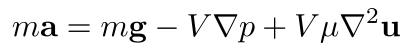
We call this the Navier-Stokes momentum equation. It says that for any fluid particle in our model, its mass times its acceleration equals its weight, plus its pressure gradient force (the minus sign is because the pressure gradient vector points from low to high pressure, while the pressure gradient force pushes particles from high to low pressure), plus its viscous force. Now, we mentioned that volume is a strange quantity to apply to fluid particles. Let's divide the whole equation by the particle's mass, which we assume is strictly positive (i.e., we're not dividing by zero!), and note that density is ρ = m/V, and thus V/m is 1/ρ:

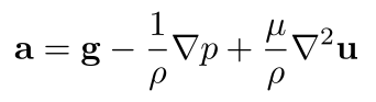
Let's also replace μ/ρ with a new symbol, known as the coefficient of kinematic viscosity, ν (the Greek letter "nu"):

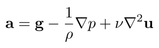
Unsteadiness & Advection

Now, it may seem like we're done, but to actually compute fluid flow, we need fluid velocity, not acceleration. Well, that's easy, isn't acceleration just the time-derivative of velocity? Sure, but there's an important detail relating a fluid particle's acceleration to its velocity that we need to handle: the concept of advection. In a nutshell, advection just means "moving" and carrying some quantity with you as you move. The term actually has a more specific meaning in fluid dynamics and vector calculus. Dr. Bridson and Dr. Müller-Fischer's course notes and Dr. Matthew Juniper's fluid dynamics notes both explain this really well. But here's a brief description.

The temperature at any point in Earth's atmosphere can change for many reasons. On a sunny day, solar radiation from the Sun can get absorbed by the ground and then transferred to the air above it, which then increases the temperature of air at any point in that area. But then, a cold front could plow through, cooling the air at any point in that area. These are two very different mechanisms for changing the temperature at any given point in the atmosphere. The first is an external heat source causing a general increase in the temperature of all air parcels in some area, even if none of the air is moving. The second is the air itself, carrying cooler temperatures with it and pushing the warmer air out of the way. This second mechanism is called advection: it's when cooler air displaces warmer air, changing the temperature at a fixed location in space simply by air moving around. The first mechanism is called unsteadiness--a general change in the temperature field that occurs even if no air ever moved anywhere. Unsteadiness is your shirt changing color due to the lighting around you changing, while you sit perfectly still. Advection is you wearing a bright red shirt and changing the spatial distribution of redness in the world by running around with that bright attire. Unsteadiness is change of a quantity (like temperature or color) at a fixed point in space without motion; advection is change of that quantity at a fixed point in space solely due to motion.

Well, any field can technically be advected, including the fluid velocity itself! You can imagine that if the water in a lake was sitting perfectly still, a boat's propeller could start spinning and push the water to change its velocity at any specific point around the propeller. This is "unsteadiness" since the fluid velocity at a specific point changed due to some external velocity-changing mechanism (the propeller in this case). On the other hand, if some fluid particles already were moving faster than others, then at a specific point in space, the overall flow of the water would carry faster particles into some areas and slower particles into other areas. This is advection: a change in the water velocity at a given point in space due simply to the fluid's own motion carrying fluid particles of various speeds around, and not because some external agent was accelerating the fluid at that point.

Mathematically, we can start by just saying, acceleration is the time-derivative of the velocity of the fluid. Since fluid velocity is a function of x, y, z, and t, and since the first three of these variables are also functions of time (i.e., the coordinates of a moving fluid particle), we apply the chain rule to get that the overall derivative of fluid velocity, often referred to as the total or material derivative, Du/Dt, is:

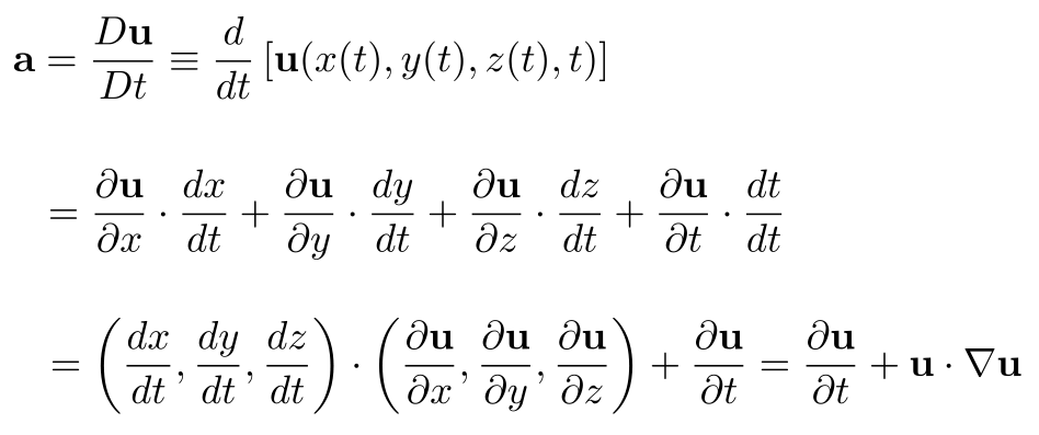
These terms are precisely what we talked about above: the first term, ∂u/∂t, is the unsteadiness term describing local changes to the fluid velocity at any point independent of the fluid's motion and the second term, u · ∇u, is the advection term, describing the change of the fluid's velocity at any given point due solely to the fluid's motion i.e., the fluid velocity, i.e., the instantaneous change to the fluid particle's position, (x, y, z).

Final Form of the Navier-Stokes Momentum Equation

Replacing a in our most recent version of the Navier-Stokes momentum equation with this unsteadiness term plus advection term gives us the final form of the Navier-Stokes momentum equation we'll use for simulation:

In computer graphics, it's common to assume zero viscosity, i.e., to remove the viscous force term from the Navier-Stokes momentum equation. That gives us the inviscid approximation to the Navier-Stokes momentum equation, the Euler momentum equation,

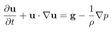
In this tutorial, we'll stick with this inviscid approximation of the Navier-Stokes momentum equation.

Mass Conservation & Incompressibility

The derivative of the fluid pressure function for a given parcel of fluid (a box-shaped particle) can be approximated to up to its first-order term in its Taylor series as Dr. Matthew Juniper's fluid dynamics notes explain, along with an assumption that fluid mass is conserved within any arbitrary volume of fluid (an application of the law of conservation of mass we stated earlier as a fundamental assumption of physics), to derive an equation called the equation of mass continuity. Alternatively, using the Divergence Theorem, the same equation can be derived:

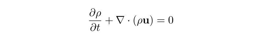
Following the derivation here, assuming the fluid density function is constant within the infinitesimal volume of a fluid parcel that flows with the fluid, i.e., Dρ/Dt = 0, we obtain the incompressibility condition:

The Navier-Stokes momentum equation taken together with the incompressibility condition (which itself is just the law of mass conservation with constant material density) are often simply called the Navier-Stokes equations. In our case, since we're neglecting viscosity, the Euler momentum equation (the inviscid Navier-Stokes momentum equation) together with the incompressibility condition are called the Euler equations.

Splitting

As described in Bridson and Müller-Fischer's SIGGRAPH 2007 course notes and Robert Bridson's book on fluid simulation, we will use this equation to simulate a fluid by splitting it up into parts and handling each part separately. Overall, our strategy will be to start with an initial fluid velocity field, u(x, y, z, 0), that has zero divergence. We'll then keep computing new velocity fields at successive time steps, u(x, y, z, Δt), u(x, y, z, 2Δt), u(x, y, z, 3Δt), etc. But note that our goal is to make sure all of these velocity fields at each of these time steps have as close to zero divergence as possible.

To do this, we will follow a procedure similar to that in Section 2.2 of Bridson and Müller-Fischer's SIGGRAPH 2007 course notes, with a few changes, such as keeping a constant time step size, Δt. Here is our procedure:

• Initialize the time t = 0.
• Start with a zero-divergence velocity field u(x, y, z, t).
• For the duration of the simulation:
  • Set u = Advect(u(x, y, z, t), Δt).
  • Set u += Δtg.
  • Set u = ProjectPressure(u, Δt) such that u has approximately zero divergence.
  • Set t += Δt.

These steps are just adding the advection term, gravity term, and pressure gradient term to the unsteadiness term, i.e., the partial derivative of the fluid velocity with respect to time, in the inviscid Euler momentum equation.

The next several sections will build up a complete implementation of a fluid simulator. First, we'll describe a data structure that stores the scalar and vector fields like pressure, density, and velocity in a digital form as a 3D staggered grid of data values covering a region of space containing our fluid(s) of interest. Then we'll explain how we exchange data from this grid to individual particles that carry position and velocity information with them. We'll then apply the steps above to contribute the effects of advection, gravity, and pressure to the fluid velocity values stored by our particles. We'll then show how we map particle data back to the staggered grid. This process will be repeated in every time step until we reach the end time of our simulation.

The Staggered Grid

Fluid simulations involve a data structure called the staggered grid or the marker-and-cell (MAC) grid. The staggered grid separates points where we sample each of the four following values: fluid pressure and the x, y, and z components of fluid velocity. This will help us calculate derivatives of pressure and velocity for physics-based simulations of fluids. See Robert Bridson's excellent book on fluid simulation for details on the staggered grid data structure. An explanation of the staggered or MAC grid is in Section 2.4 of Bridson and Müller-Fischer's SIGGRAPH 2007 course notes.

Staggered Grid Structure

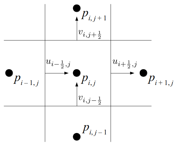
The staggered grid is a 2D or 3D grid representing the full spatial volume within which we simulate our fluid(s). We will label each grid cell of a 2D staggered grid with a row (along the x direction) index, i, and a column (along the y direction) index, j:

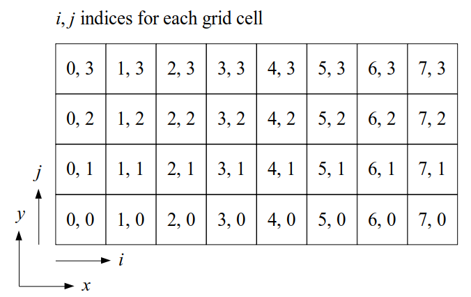
At the center of each grid cell with indices i and j, we will store a nonnegative fluid pressure value, p_{i, j} ∈ R. At the center of each boundary between adjacent grid cells, we will store a component of the fluid velocity that's perpendicular to that boundary. That is, at the center of the boundary between grid cell i, j and grid cell i + 1, j, we store the horizontal component, u_{i + ½, j} ∈ R, of the fluid's velocity at that location. At the center of the boundary between grid cell i, j and grid cell i, j + 1, we store the vertical component, v_{i, j + ½} ∈ R, of the fluid's velocity at that location:

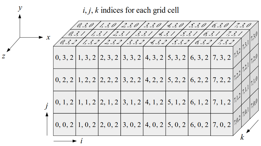
We will label each grid cell of a 3D staggered grid with an index i along the x direction, index j along the y direction, and index k along the z direction:

Like the 2D staggered grid, the 3D staggered grid will have a fluid pressure value, p_{i, j, k}, stored at the center of each grid cell with indices i, j, k. At the center of each boundary face between adjacent grid cells, the 3D grid will also have a component of the fluid velocity perpendicular to that boundary:

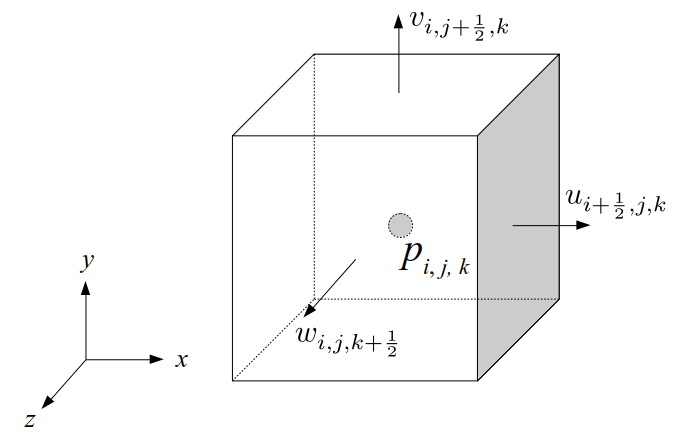
Note that for both the 2D and 3D staggered grids, the velocity components are not components of a single 2D or 3D velocity vector! Instead, we are storing different components of the fluid velocity at entirely different locations in space.

Storing Staggered Grid Data

We will focus on implementing the 3D staggered grid, although we'll start with a 2D grid description since it's much easier to understand the main concepts and then extend to 3D than to see the concepts for the first time in 3D. As you can see, we need to store a variety of values in some kind of 3D array. For example, we need to store the fluid pressure for any given grid cell with indices i, j, and k. We also need to store the u, v, and w values, i.e., the x, y, and z components of the fluid velocity at the appropriate grid cell boundaries. We will also need to store non-real-number values, e.g., whether each grid cell contains a solid or fluid or is empty.

We will begin by creating a class, Array3D, based on the class of the same name in Bargteil and Shinar's SIGGRAPH course. The Array3D class will be templated so we can use it to store different types of data, e.g., double values for real numbers like pressure and velocity and other data types for labeling grid cells as containing solid or fluid or being empty. But exactly how large should our 3D array be for each type of value? For example, the velocity components are defined at the grid cell boundaries rather than at the cells themselves and we do this weird indexing of them with "½" thrown in just to make life difficult?! Let's do a quick illustration to make sure we count this properly.

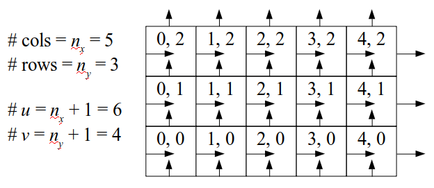
Assuming we store velocities not only between grid cells but really on all faces of grid cells, i.e., including the boundary of the entire grid, we will actually end up storing differently-sized arrays for different quantities. If we define n_x as the number of columns of our grid, i.e., i ∈ {0, 1, ..., n_x - 1}, and define n_y as the number of rows in the grid, i.e., j ∈ {0, 1, ..., n_y - 1}, then it's easy to see from the diagram above of a 2D grid that the number of horizontal velocity components we store is (n_x + 1)n_y while the number of vertical velocity components we store is n_x(n_y + 1). Meanwhile, the number of pressure values we store would just be one per grid cell, i.e., n_xn_y. Any array of labels we store for each grid cell would also be of that size, n_xn_y.

Extending this to 3D, the i and j indices have the same range as above, and with n_z representing the depth (number of grid cells in the z direction) of the grid, k ∈ {0, 1, ..., n_z - 1}. I hope I have convinced you that the 3D array of pressure values would be a n_x ✕ n_y ✕ n_z array. The 3D array of horizontal velocity components would be a (n_x + 1) ✕ n_y ✕ n_z array, the vertical components would be a n_x ✕ (n_y + 1) ✕ n_z array, and the depth (z direction) components would be a n_x ✕ n_y ✕ (n_z + 1) array.

First, we'll create a basic 3D array class that can take on any reasonable nonnegative integer value (up to the range covered by the type std::size_t in C++) for each of its three dimensions. The Array3D class will be templated so we can store values of any data type inside it. We will start with just a constructor, an accessor ("getter") function that allows us to look up a value at a particular i, j, k index in the array without modifying it, and a mutator ("setter") function that does the same thing as the accessor but allows us to change the value if we want. We'll also add accessor ("getter") functions that return the dimensions, n_x, n_x, and n_x of the array. Note that all of this code will be implemented in a single header file, Array3D.h (as is typical for templated classes, there is no associated .cpp file). I put this into a new subdirectory of our code called incremental0. The next several files of C++ code we create will also go into this same subdirectory. We could dump everything into one directory, but this way we can isolate the different stages of our code development into smaller pieces.

Note we declared the copy constructor and assignment operator as private without implementing them; this prevents accidental misuse of any default copy constructor or assignment operator by any code outside of this class (e.g., code that instantiates and uses this class), reducing the chance of unintended bugs when using this class. We also require that nx_, ny_, and nz_ are constants: they get initialized upon construction of an Array3D object and will never change during the life of the object. The object's data is deleted upon destruction. To test this class and demonstrate how to use it, we create a short file, Array3DTest.cpp, also in the incremental0 directory.

To compile and run both Array3DTest.cpp and Array3D.h, we issue these two commands while we are in the incremental0 directory:

g++ Array3DTest.cpp -o Array3DTest
./Array3DTest

This results in the following output:

Array is 3 x 4 x 5.

table(0, 0, 0) = 7
table(1, 3, 4) = 12

This is what we expected! We created a 3 ✕ 4 ✕ 5 array of integers, assigned 7 to the value at index 0, 0, 0, assigned 12 to the value at index 1, 3, 4, and then looked up the values those two indices and retrieved them, verifying that our mutator and accessor functions seem to be doing what we intended. To clean up after running this test program, I recommend:

rm Array3DTest

Let's leave the Array3D class implementation aside now that we have a basic functionality in place. We'll revisit how to change or add to this class as needed when we implement a fluid simulation algorithm.

But how do we represent the velocity component arrays using the Array3D data structure? Array3D only accepts integer indices as inputs to its accessor and mutator functions, yet all the indices we use to refer to the velocity components in the staggered grid have ½ in one of the three indices? We use the convention Bridson and Müller-Fischer describe (see, for example, Slide 46 of this presentation). Recall the horizontal components, u, of fluid velocity will be stored in a 3D array with dimensions (n_x + 1) ✕ n_y ✕ n_z. The 3D array for u values in the 3D staggered grid can have u(i, j, k) = u_{i - ½, j, k}, for all values of i from 0 through (n_x + 1) - 1 = n_x . So, u(0, 0, 0) = u_{-½, 0, 0}, u(1, 0, 0) = u_{½, 0, 0}, and u(nx, 0, 0) = u_{nx - ½, 0, 0}. Going from i = 0 through i = n_x adds up to a total of n_x + 1 cells in a row of the grid. Similarly, for all values of j from 0 through n_y, v(i, j, k) = v_{i, j - ½, k}. And for all k from 0 through n_z, w(i, j, k) = w_{i, j, k - ½}. In contrast, a 3D array to store fluid pressure values will just have the same dimensions as the grid itself: for i ranging from 0 through n_x - 1, j ranging from 0 through n_y - 1, and k ranging from 0 through n_z - 1, p(i, j, k) = p_{i, j, k}.

The Staggered Grid Data Structure

Now we can put together a basic staggered grid class that contains 3D arrays, as described above, to store pressure values and velocity component values. Here are the header file, StaggeredGrid.h and the implementation file, StaggeredGrid.cpp. We also create a small test program in another file, StaggeredGridTest.cpp. All of these files are also in my incremental0 directory.

We compile this with the following command:

g++ StaggeredGrid.cpp StaggeredGridTest.cpp

Note that both the class definition file, StaggeredGrid.cpp, and test program file, StaggeredGridTest.cpp, must be compiled together. If you only compile the test program, you will get undefined reference errors because the C++ compiler won't be able to find the implementations of the constructor and destructor that are in StaggeredGrid.cpp. Next, run the resulting program:

./a.out

The output should look like:

Created StaggeredGrid:
- p array is 3 x 4 x 5
- u array is 4 x 4 x 5
- v array is 3 x 5 x 5
- w array is 3 x 4 x 6

This matches what we expected: the original grid was 3 ✕ 4 ✕ 5. The horizontal velocity grid has one more horizontal component than the original grid, so it's 4 ✕ 4 ✕ 5. Similarly, the vertical and depth velocity grids also have exactly one dimension with one more slice than the orignal grid.

Grids vs. Particles for Fluid Simulation

We haven't fully clarified why we use a staggered grid for fluid simulation other than something about better derivative-taking. This will get clearer as we flesh out the complete algorithm we'll be implementing for fluid simulation. Critical to our approach is using not only this staggered grid, but also particles in the spirit of what we did earlier when simulating Newtonian mechanics using spheres. What is this madness? We use particles and grids? To do what exactly?

Let's back up a little more before we continue onto more details of our simulation approach. How do you use a computer to simulate the physics of fluids? As we've seen earlier, we can simulate individual particles that feel forces and bounce off of the walls of the viewing frustum and bump into each other. But, it's also common to use grids to simulate fluids--instead of individual particles, you can just keep track of fluid properties like velocity and pressure at specific, fixed points on a grid in space, and not have to track individual particles.

But there are pros and cons to both particles and grids. As explained, e.g., on Page 5 of Bridson and Müller-Fischer's 2007 SIGGRAPH course notes, the grid-based, or Eulerian, approach to fluid simulation is much better for calculating derivatives with respect to spatial coordinates--it's easier to calculate Δx on a fixed grid (you know where the xs are at all times) than over a cloud of constantly moving particles (the xs keep moving all over the place). On the other hand, simulating a fluid as a bunch of individual particles (the Lagrangian approach) makes some things easier--Newton's laws apply directly to each particle and if each particle has a fixed mass and the number of particles stays constant during a simulation, then mass is automatically conserved.

Fluid simulation, for the most part, focuses on the Eulerian (grid-based) approach rather than the Lagrangian (particle-based) approach since a fluid is often best modeled as a continuum with variables like velocity and pressure that change over time. Historically, simulating a fluid as thousands or millions or billions of particles was computationally too difficult anyway. But, since there are also some advantages to the particle-based approach, a common approach to fluid simulation these days is to mix the two approaches into a semi-Lagrangian approach, where you do some calculations on particles, then map values from the particles to the grid, do some calculations on the gird, and then map values from the grid back to the particles, and repeat. These simulation methods that use both particles and grids are generally called "hybrid" methods, since they blend Eulerian (grid) and Lagrangian (particle) viewpoints.

The specific type of fluid simulation algorithm we'll introduce in this tutorial is called the Fluid Implicit Particle (FLIP) method. FLIP is a class of fluid simulation algorithms that resulted from early research in the mid-20th century on fluid simulation. See Bridson and Müller-Fischer's notes and the associated book for more details. A very nice introduction to the trade-offs in FLIP vs. other "hybrid" particle-grid methods is given in a paper by Ding et al. (2019).

Mapping from Particles to the Grid

We'll build up the componenets of the specific implementation of FLIP presented in and provided with Bargteil and Shinar's 2019 SIGGRAPH course mathematically and visually first. Then we'll build up the actual C++ code to implement a modified version of the specific version of the FLIP method provided with that SIGGRAPH course.

One part of our FLIP algorithm will involve transforming velocities of particles into velocity components on the staggered grid that we'll use for fluid simulation. Our velocity component 3D arrays in our staggered grid will all be zeroed out first. We'll pretend that each particle isn't really just a zero-dimensional point; rather, each particle will be like an object with some real power and influence over the grid cells around it, and we'll take each particle's velocity and splat (yes, that's a technical term, see this page for example) the particle velocity onto neighboring grid cells' velocity components to make our 3D arrays of velocity components then represent a sort of Eulerian "field" of fluid velocities. We'll explain later why we do this, when we do this in each time step of our simulation, later. Here I just want to highlight some minute details of the indexing and mapping process so we don't get confused trying to write the code for this part later.

Barycentric Weights of a Particle

Since a grid has to exist somewhere in space and have some fixed size for its grid cells, let's denote the location of the lower corner of the grid, i.e., the point with the lowest value of x, y, and z in the entire grid, as l_c (yes, that's a lowercase letter "ell" for "lower" and then subscript "c" for "corner"). Let's assume each grid cell is a perfect cube with all side lengths equal to some nonzero real number Δx; yes, even in the y and z directions, not only the x direction.

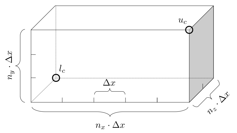
The figure above shows the lower corner, l_c, the upper corner, u_c (the point with the greatest x, y, and z coordinate values in the entire grid), and the grid spacing, Δx. Recall that the number of grid cells in the x dimension is n_x, the number of cells in the y direction is n_y, and the number of cells in the z direction is n_z, so u_c = l_c + (n_x + Δx, n_y + Δy, n_z + Δx).

Note that l_c and u_c can be literally any two points in R³ as long as u_c's three coordinates are greater than l_c's respective three coordinates. But we index our grid cells using integers: i, j, and k. So we'll need a way to translate between the integer cell indices and the actual real-number coordinates of any location of a particle within the grid. Let's start with this question, which we'll need to answer to implement our FLIP algorithm: given an arbitrary particle p located at some point (x, y, z) in this grid, what are the indices, (i, j, k), of the grid cell that contains p, and relative to that grid cell's lower corner, how far into the grid cell in each coordinate direction is the particle's location, relative to the grid cell width?

To figure that out, it's actually easier if we note that the computation of indices of a grid cell containing a particular point is independent in each coordinate direction. That is, the i index of the cell containing p is only dependent on x (i.e., p's x-coordinate), j only depends on y, and k only depends on z. So, very briefly, let's just imagine we only had a one-dimensional grid: basically a finite-length interval of the real number line whose leftmost position is l_c's x-coordinate and whose rightmost position is u_c's x-coordinate.

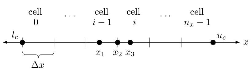
The figure above illustrates a one-dimensional (1D) grid extending from some real number l_c to another greater real number u_c. There are n_x grid cells, each with width Δx. So u_c = l_c + n_x · Δx. If a point is strictly inside the boundaries of a grid cell, then we consider that cell to be the cell that contains it. If a point is on the boundary of a grid cell, we consider it to be in the grid cell that extends to the right of the point. So, l_c is in cell 0, x₁ is in cell i - 1, and x₃ is in cell i. x₂ is in cell i since the point is on the left boundary of that cell.

So if the only known values are l_c, Δx, and n_x, then if we are given a particular point x, how can we determine which grid cell contains x? Here is our procedure:

1. Subtract the lower bound, l_c, from the point's value, x, to get the 1D vector displacement, x' = x - l_c, of the point relative to the grid's lower corner.
2. Determine how many "grid cell displacements" it takes to get to the grid that contains the point x from the lower corner l_c. This is just ⌊ x' / Δx ⌋. That is, the floor of (greatest integer less than or equal to) x' / Δx, or equivalently, the result of dividing the displacement x' by Δx and throwing away the remainder. This is, in fact, just the index i of the grid containing x. So, i = ⌊ x' / Δx ⌋. Plug in some known values to verify. For example, if x = l_c, then x' / Δx = (x - l_c) / Δx = (l_c - l_c) / Δx = 0, the floor of which is 0, the correct index of the cell containing l_c. If x = l_c + Δx/2, then i = x' / Δx = (x - l_c) / Δx = (Δx / 2) / Δx = ½, the floor of which is also 0, the correct index of the cell containing the point. You can plug in values of x like l_c + Δx, l_c + 3Δx/2, and so on, to convince yourself that this calculation works for all possible values of x within our 1D grid. For now we'll ignore the fact that u_c would, by this scheme, end up in some nonexistent grid cell with index n_x.

Once we've determined which grid cell contains x, the second part of our question was, how do we characterize how far into that grid cell x is, relative to the width of a grid cell? Note that the left end of the grid cell with index i is just l_c + i · Δx. The displacement from that point to the right end of the grid cell is just another Δx to the right. Okay. So if we were exactly at the midpoint of grid cell i, then we'd be at the point x = l_c + i · Δx + Δx / 2. If we were only one-fourth of the way into grid cell i from the cell's left boundary, we'd be at the point x = l_c + i · Δx + Δx / 4. If we were three-fourths of the way into the grid cell, we'd be at x = l_c + i · Δx + 3 Δx / 4. So, the overall pattern, then, is that if we are a fraction w₀ into grid cell i, then we are at x = l_c + i · Δx + w₀ · Δx. We call w₀ = (x - l_c - i · Δx) / Δx the barycentric weight, or just the weight for short, of the point x in the grid cell i. This is illustrated in the figure below.

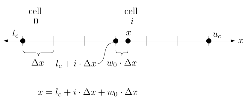
I know that probably seemed unnecessarily wordy, but it's important to get the details right, avoiding off-by-one errors, etc., and it's easier to make sure we're doing that right in one dimension than in multiple dimensions. We can actually think of what we just did as a transformation from Cartesian coordinates, x, to an index and barycentric coordinate pair, (i, w₀) = (⌊x - l_c⌋ / Δx, (x - l_c - i · Δx) / Δx) = (⌊x'⌋ / Δx, (x' - i Δx) / Δx) = (⌊x'⌋ / Δx, x' / Δx - i). Now, let's extend this quickly to two dimensions.

Let's now extend this to two dimensions. Knowing that all the math works out identically for x and y coordinates, we can derive our transformation from Cartesian coordinates of a particle's 2D position, (x, y), to its cell indices (i, j), and barycentric weights, (w₀, w₁). Let's first subtract l_c's coordinates (note l_c is now a point in R² with 2 coordinates, not just a single real number) from the particle's 2D position to get the particle's displacement relative to l_c, which we'll denote as (x', y') = (x, y) - l_c. Then i = ⌊x'⌋ / Δx. Similarly, j = ⌊y'⌋ / Δx. As before, w₀ = x' / Δx - i. Similarly, w₁ = y' / Δx - j. This is illustrated in the figure below.

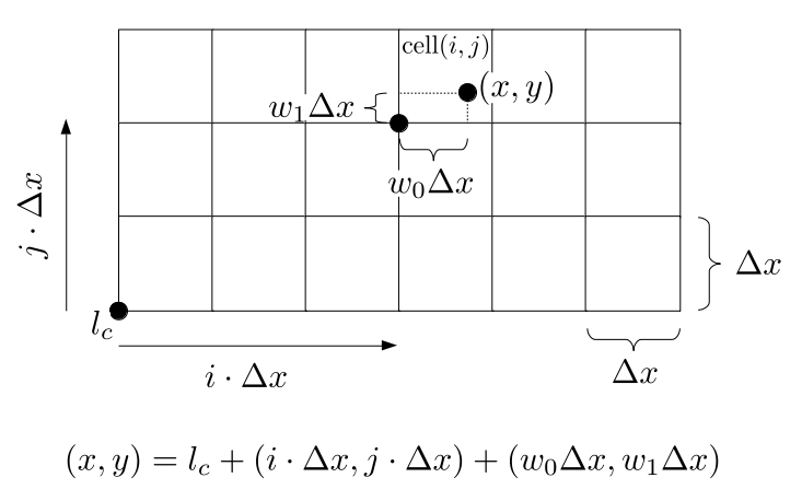
Now going all the way to three dimensions, a particle at (x, y, z), or relative to the lower corner of the grid, (x', y', z') = (x, y, z) - l_c, will have indices

• i = ⌊x'⌋ / Δx
• j = ⌊y'⌋ / Δx
• k = ⌊z'⌋ / Δx

• w₀ = x' / Δx - i
• w₁ = y' / Δx - j
• w₂ = z' / Δx - k.

This is illustrated in the figure below. This is the set of calculations we'll use for our fluid simulation algorithm since we are mostly interested in simulating fluids in 3D, not 2D or 1D.

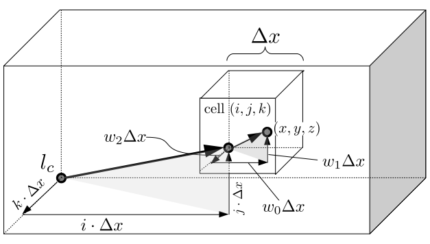
Note that we can think of this as a breakdown of a point's position as starting from the lower corner, l_c, translating by (i · Δx, j · Δx, k · Δx), and then translating once more by (w₀ · Δx, w₁ · Δx, w₂ · Δx) to get to a particle's position, (x, y, z). We can even think of this as follows: if we translate the entire grid so that the lower corner, l_c ends up at the origin and then scale the entire grid so that Δx becomes 1, then the actual coordinates of the point (x, y, z) become (i + w₀, j + w₁, k + w₂)!

Note that Δx is technically just a positive real number, but sometimes when we label a vector with it like in the figure above, we're imagining it representing a vector with a length equal to what the label says, pointing in the direction of that arrow.

Let's now implement two functions: one to compute i, j, and k for a given particle position and another to compute the barycentric weights, w₀, w₁, and w₂. Let's call the first function floor following Bargteil and Shinar's code. The function will take as input a point, (x, y, z), a lower corner point, l_c = (x_lc, y_lc, z_lc), and a grid cell width, Δx, and return three integers, i, j, and k, indicating the indices of the grid cell containing that particle, according to the calculations shown earlier. But wait! How are we going to represent all this data in C++? How will we return 3 integers from a function all at the same time?

Our grid spacing (grid cell width) parameter, Δx, can just be a double as in Bargteil and Shinar's code. But how will we represent the two 3D point parameters, (x, y, z) and (x_lc, y_lc, z_lc)? Well, we could create our own 3D point data type, or, we could just use the Eigen library, as Bargteil and Shinar's code does. While we attempt to minimize the number of external libraries we insert into this tutorial's code, Eigen is so standard in graphics and physics-based computing that importing it is really not a burden. And it's very easy to install and use. Not to mention, it has some performance advantages, such as lazy evaluation, where it does as much manipulation of algebraic expressions involving vectors and matrices at compile time as it can, minimizing the amount of computation done at run time.

To install Eigen, if you haven't already, run this command in a terminal:

sudo apt install libeigen3-dev

Then type this command to figure out where Eigen was installed:

whereis eigen3

For me, this command returned /usr/include/eigen3. Remember this or write it down somewhere, since we will use this path to compile any code that uses Eigen.

Let's also answer the other question from earlier: how will we return three integers from a function all at the same time? Well, we could just pass the integers in by reference and let the function modify them in order to "return" them without really returning them. However, this has some issues as we shall see soon. Here's one way to implement this function a not-so-great way, in a complete program with a main() function for some quick sanity-checking of our code's correctness, in a file I called GridIndexing_Bad.cpp, still in our incremental0 directory.

Note we just used casting to integers to do the "floor" operation of finding the largest integer less than or equal to a given double-precision number. This works when the value is known to be positive, as is the case for us here (it wouldn't work that way for negative numbers, though!). Compile this code with this command, which includes the Eigen path noted above, and doesn't unnecessarily include the OpenGL library stuff since we're just doing a simple math operation using vectors:

g++ GridIndexing_Bad.cpp -o GridIndexing_Bad -I/usr/include/eigen3/

Run the code with:

./GridIndexing_Bad

Here's the output:

i = 2, j = 1, k = 0
i = 3, j = 8, k = 9
i = -1, j = 0, k = 0

There are several issues with this implementation. First, you may notice that last call to floor results in a negative index, which makes no sense! Also, what if dx, i.e., Δx, had been zero, or negative? There's nothing in the code preventing that from happening! Also, doesn't it seem weird that we use some special data type, Eigen::Vector3d, to handle a 3D vector of doubles, but we just use three separate integer variables to handle essentially a 3D vector if ints?

The floor function has an issue which is often not considered a problem by many: it is stateful, meaning it takes in some variables from outside its scope and alters them. Instead, stateless functions (e.g., that simply take in parameters and return other values, acting in total isolation from all other code) are preferable to stateful ones (e.g., functions that take in references or pointers to variables and then modify them) for a variety of reasons. And in C++, we usually don't have to worry about extra copies of returned objects slowing down our code since a standard optimization C++ compilers use is return value optimization. So, let's create a simple data structure representing a triplet of nonnegative integers, (i, j, k), and have the value returned by our floor function be an instance of that data type.

So, we can make some improvements to our code in a new file, GridIndexing.cpp in our incremental0 directory.

Compile and run your code the same way, but without the _Bad suffix because well, now our code is not as bad, apparently. Note we're not actually compiling our code using compiler optimizations yet. We'll do that later when we get to some heavier computation. The program should output some text and then crash on an assertion failure since it, correctly, disallows negative indices:

Indices: 
2
1
0
Indices: 
3
8
9
GridIndexing: GridIndexing.cpp:33: GridIndices floor(const Vector3d&, const Vector3d&, double): Assertion `p_lc_over_dx[0] >= 0.0' failed.
Aborted (core dumped)

Now that we've finished computing the index of the grid cell that contains any given particle position, let's work on implementing the function to compute the barycentric weights of a given point. To determine the weights of a particular particle position, as we saw above, we do need to know which cell contains it. The floor function we just implemented does exactly that. Let's use the indices returned by the floor function as inputs into our barycentric weight calculator function, which we'll call weights, following Bargteil and Shinar's code. Let's again make the function stateless, which is a bit different from their implementation. So, the function will have as input the particle position, the grid's lower corner point, the grid spacing, and the indices of the cell containing the particle's position. The value we return this time will be a 3D vector of doubles, which are the barycentric weights of the particle position's in that cell.

Notice here that we'll be repeating some calculations here, like the subtraction of the particle's position by the grid's lower corner position and division of all of that by the grid spacing. But we'll deal with that inefficiency later when we get to a more complete program; for now, let's implement this function with the parameters we described above, in a little test program called GridWeights.cpp, still in the incremental0 directory.

Compile and run this code the same way we did with the last two files. The output is:

Indices: 
0
3
4
Weights = 
0.5
  0
0.5

Indices: 
 3
 4
16
Weights = 
0.5
0.5
  0

Indices: 
0
0
0
Weights = 
0
0
0
          

That completes our work on the theory and implementation of the grid cell index and barycentric weight computation!

Notice we declared the floor and weights functions as inline, as in Bargteil and Shinar's code. This isn't necessary to do for these little test programs, but does promote efficiency in larger programs by making the compiler do the work of basically replacing any call to these functions with the actual code inside the functions to avoid an extra function call being stacked onto the call stack of our running programs.

Splatting Particle Velocities onto the Grid in 2D

Now that we know how to break down a particle's position into its grid cell's indices and the barycentric weights of its location within the grid cell, let's look at one important step of the FLIP algorithm: splatting the particle's velocity onto nearby grid velocity components. What is splatting and why do we do it?

As we mentioned earlier, in hybrid fluid simulation algorithms that use both particles and grids, we will repeatedly map from particles to the grid and from the grid back to the particles. Splatting is the process of mapping from the particles to the grid. In this case we will just focus on splatting particle velocities onto the velocity components of nearby cells in a staggered grid.

Since there will be a lot of gymnastics involving indices in the splatting process, we will go through it carefully. It can get really confusing to just look at the algorithm or implementation, without much explanation, as it is full of ws and indices with +1s and -1s all over the place. A lot of conceptual detail is actually hidden by the implementation of splatting in code form, so we'll break it down here and then build up the implementation in C++ after completing our understanding of the algorithm mathematically.

The general idea of splatting is that every particle has some influence over not only the grid cell it is currently in, but also potentially some neighboring grid cells. We get to define exactly how much influence the particle has over the velocity components of neighboring grid cells and how big that neighborhood even is. The figure below illustrates this very general idea. It's formalizing the idea of popping a water balloon and watching the water go splat!, making a huge mess all over the unfortunate grid cells near it.

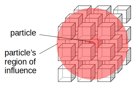
We'll build up the splatting algorithm used in the FLIP code provided with Bargteil and Shinar's SIGGRAPH course. The code defines the region of influence of a particle as follows. First, draw an imaginary grid cell around the particle's current location. Second, determine which actual grid cells' interiors overlap with that imaginary grid cell. Those are the grid cells whose velocities will be updated based on the particle's velocity. As we'll see later, the change to each velocity vector will be proportional to the amount of overlap between the imaginary grid cell of the particle and the portion of the actual grid cell that borders that velocity vector's location.

Let's start by examining a one-dimensional example of one part of the splatting algorithm. To determine the grid cells that overlap an imaginary grid cell centered on a particular particle, we do a negative shift by half a grid cell width from a particle's position; this would be the lower (left) end of the imaginary grid cell centered on the particle. The figure below illustrates this.

The shift works like this: subtract Δx/2 from the particle's location, x, and note in which cell you end up. You can convince yourself that if x is less than halfway into grid cell i, then x - Δx/2 will be in grid cell i - 1. If x is halfway or more into grid cell i, then shifting it left by a half-grid-cell-width (Δx/2) will keep it within grid cell i. Note that if x is exactly halfway into grid cell i, then shifting it left by half a grid cell width lands it exactly at the left end of grid cell i, which we still consider to be in grid cell i and not i - 1. Another way of saying this is, if the barycentric weight, w₀ of x in grid cell i is less than ½, then the left shift will land you in grid cell i - 1, while otherwise the left shift will keep you in grid cell i.

Now, let's examine a more comprehensive version of a 2D version of the splatting algorithm (the final algorithm we'll implement is only in 3D, but some aspects are easier to visualize in 2D first), which will include not only a negative half-grid-cell-width shift, but also some contributions from a particle's velocity to velocity components of grid cells within the particle's region of influence.

Let p be a particle at position (x, y) in a 2D staggered grid. Assume (x, y) is in the bottom half of cell (i, j). (Later, we'll look at the top half case.) Here is a diagram of this particle in the bottom half of its grid:

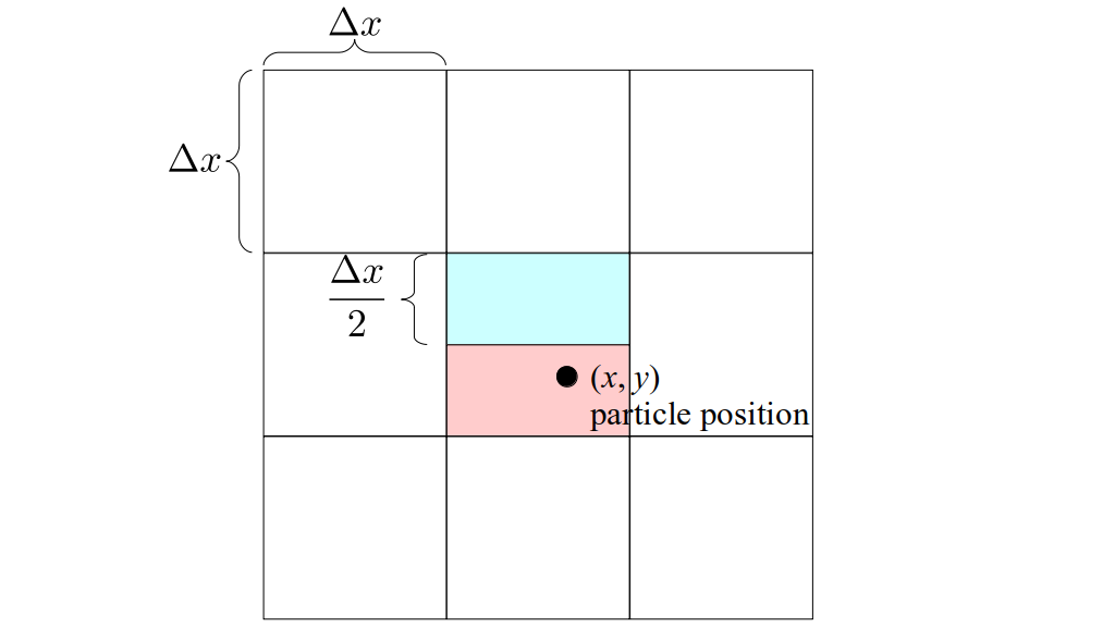
The 2D simplified version of our splatting algorithm works like this. First, shift down half a grid cell width from the particle's position to get a new position, (x, y - Δx / 2), which is located in the cell below (i, j), which is cell (i, j - 1):

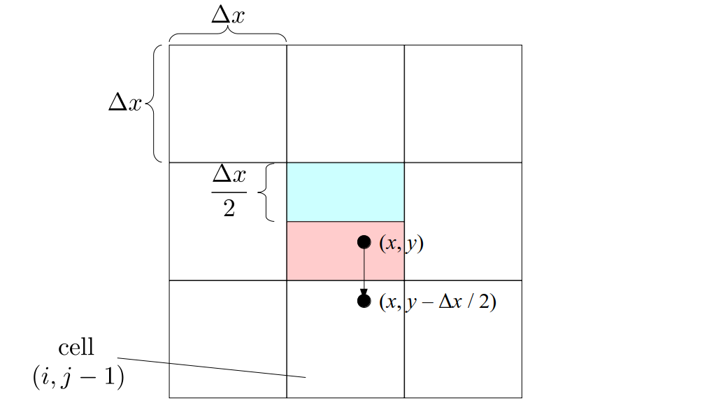
Next, compute the barycentric weights, w₀ and w₁, of that point in cell (i, j - 1):

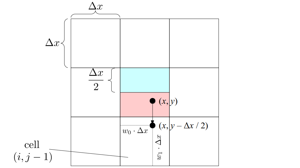
We will use those weights to splat, or contribute, weighted versions of the particle's own velocity, u_p, to the horizontal velocity components on either side of grid cells (i, j - 1) and (i, j). Here are those velocity components of those two grid cells, before splatting:

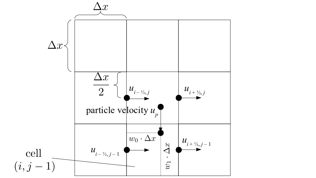
Finally, here is how the splatting works. We add (1 - w₀)(1 - w₁)u_p to the left velocity component of grid cell (i, j - 1). We add w₀(1 - w₁)u_p to the right velocity component of the same cell. For cell (i, j), we add (1 - w₀)w₁u_p to the left velocity component and w₀w₁u_p to the right velocity component:

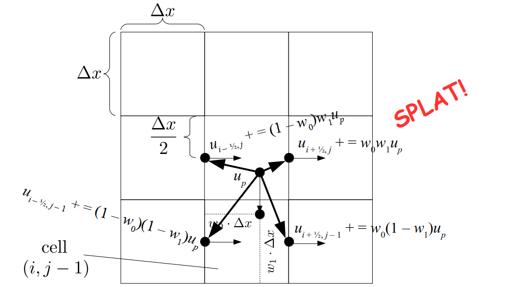
The figure above reveals how we define the "neighborhood" of the particle, i.e., the region of the grid where fluid velocities are influenced by this particle's velocity. Let's also try to get a little more intuition on what the weights are doing for us here. Notice that if the particle had been a bit more to the left (but still in the same cell), then w₀ would have been smaller. That would mean (1 - w₀) would have been bigger. But that, in turn, would mean the particle's velocity would have contributed more strongly to the left velocity components of grid cells (i, j - 1) and (i, j), since those velocity component contributions are multiplied by (1 - w₀). So, if the particle is more toward the left side of a grid cell, it contributes more to the left-side velocity components of its neighboring grid cells. That seems reasonable, right?

How does this work for the right-side velocity components? Well, if the particle is further to the right side of its grid cell, then w₀ is bigger, which means the particle's velocity contributes more to the right-side velocity components of the same grid cells since those contributions are multiplied by w₀.

What about the vertical weight, w₁? Well, the same reasoning applies. The lower the particle's position, the smaller w₁ for its downward-shifted position would be. The smaller w₁ is, the bigger (1 - w₁) is, so the more the particle's velocity contributes to grid cell (i, j - 1)'s left and right velocity components (since they are multiplied by (1 - w₁). On the other hand, the higher the particle is, the greater w₁ is, so the more the particle's velocity contributes to grid cell (i, j)'s left and right velocity components (since they are multiplied by w₁).

In fact,

Here is an animated version of this whole process:

That's it for the case where the particle is in the bottom half of its grid cell! Now, let's examine how the same process works when the particle is in the top half of its grid cell, or, exactly in the middle vertically in its grid cell (we consider both to be the same case, just as we did with the 1D shifting example above).

So, how does this process work when a particle is in the top half of its grid cell? Well, since we start higher up in the grid cell, ...

... we end up remaining in that grid cell even when we shift down by half a grid cell width:

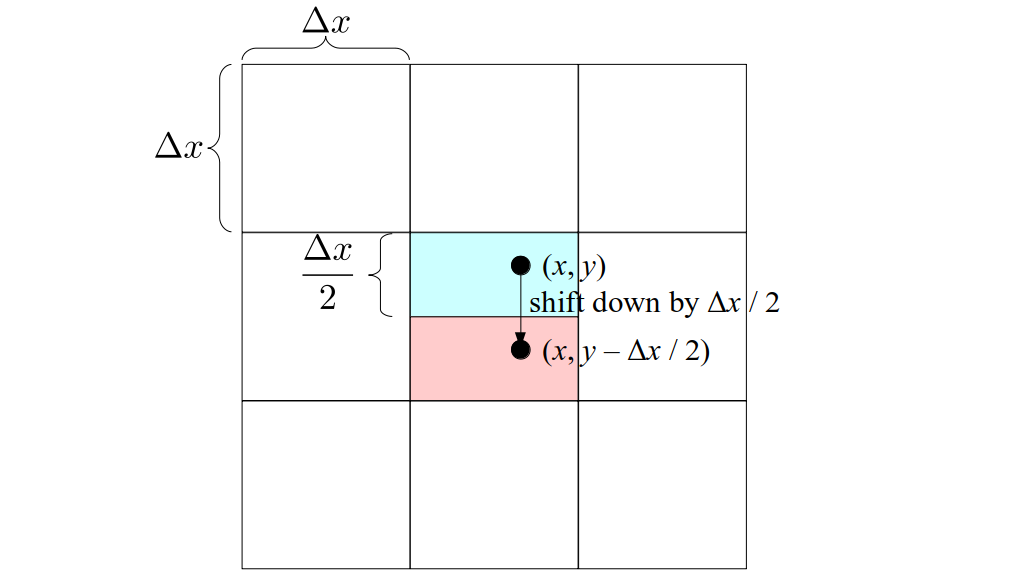
Next, we compute the barycentric weights, just like before, but relative to the cell the shifted location is in, which is the original cell (i, j), unlike in the bottom-half case above:

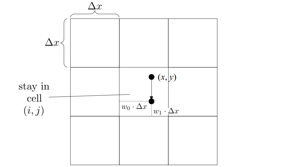
We will splat the particle's velocity onto its four neighboring velocities, as before. But unlike the bottom-half case above, we will splat the particle velocity onto the horizontal velocity components of grid cells (i, j) and (i, j + 1)! Technically we're still following the same process as before; it's just that since the downward-shifted position from the particle's position remained within the particle's grid cell, the shifted point's cell and the cell above it just happen to be a different pair of cells:

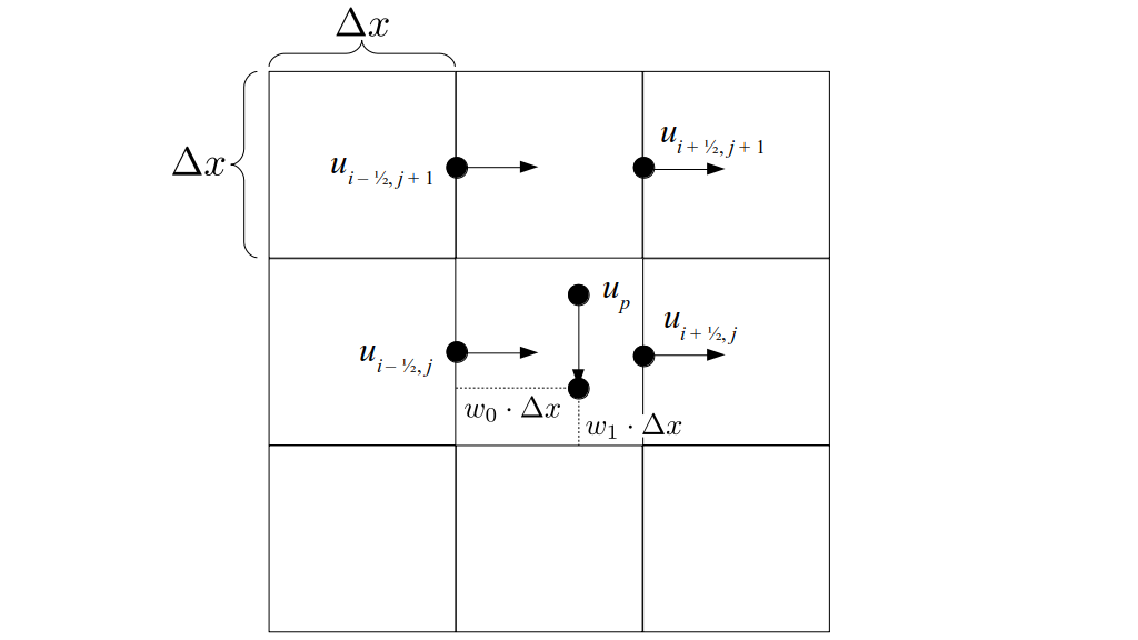
The splatting process works identically to before, but again, just on this higher pair of grid cells:

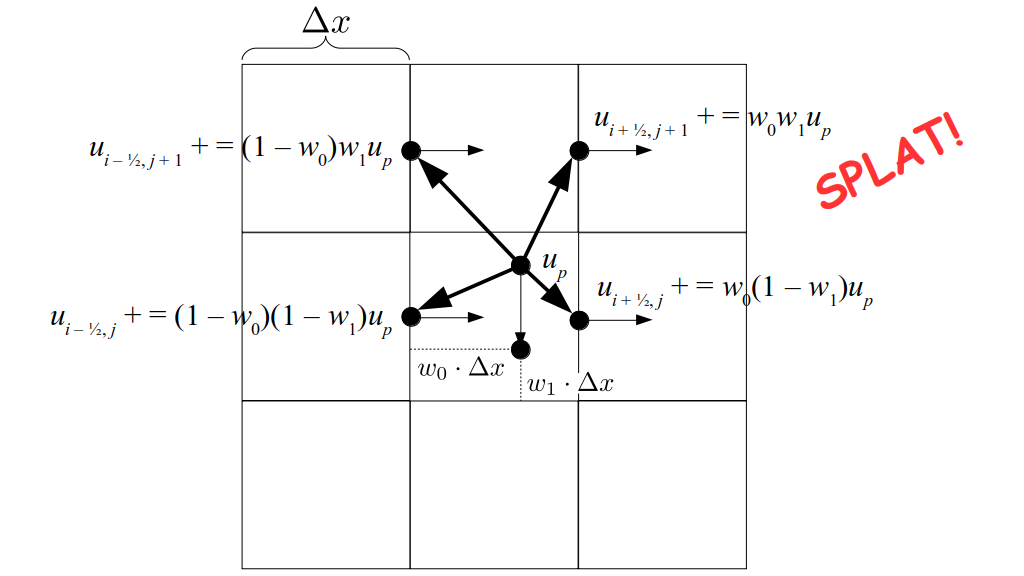
Finally, here's an animated version of this whole process for the case where the particle is in the top half of its grid cell:

Note that we can think of this process as transferring velocities from particles to every velocity on the grid; it's just that the contribution of the particle's velocity to the grid velocity components other than these four neighboring velocity components is zero.

Now, all of that gymnastics was just for splatting the horizontal velocity of the particle onto horizontal velocity components on the grid. We also have to do the same thing for the vertical components! Without going through the same level of very repetitive detail, I'll just say the process works identically in that direction; you just do a left shift by half a grid cell width instead of a downward shift, and repeat the same process.

But what exactly is this all doing? Why do we use the weights in this particular way? Is there any more insight we can get into the method behind the madness?

Well, it turns out that if you draw an imaginary grid cell centered on each of the four velocity components that get updated, and another imaginary grid cell centered on the particle's position, the fraction of the particle's velocity that each of the grid velocity components gets is exactly equal to the proportion of area overlap between the particle-centered grid cell and each velocity-centered grid cell. What?! Let's describe that a bit more slowly with pictures.

First, recall that we start with a particle position:

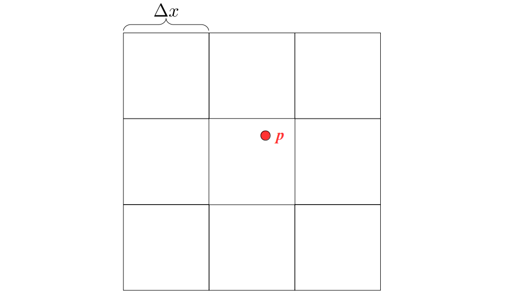
And then we shift downward by half a grid cell width and compute the barycentric weights of the resulting position in whatever cell you land:

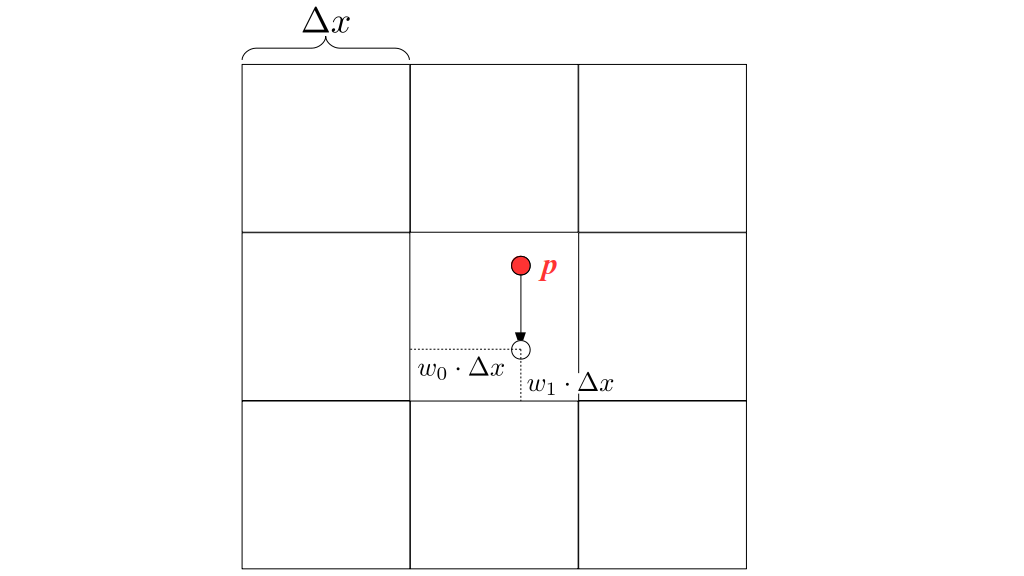
Recall that for this case, where the particle is in the top half of its grid cell, the four horizontal velocity components it'll influence are the ones next to that cell and the cell above it:

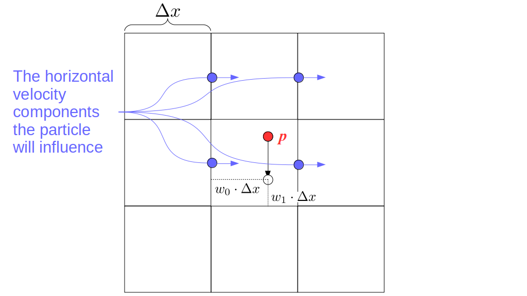
Now, draw imaginary grid cells centered at the locations of those four velocity components:

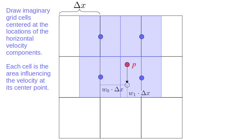
Then draw an imaginary grid cell centered on the particle's position:

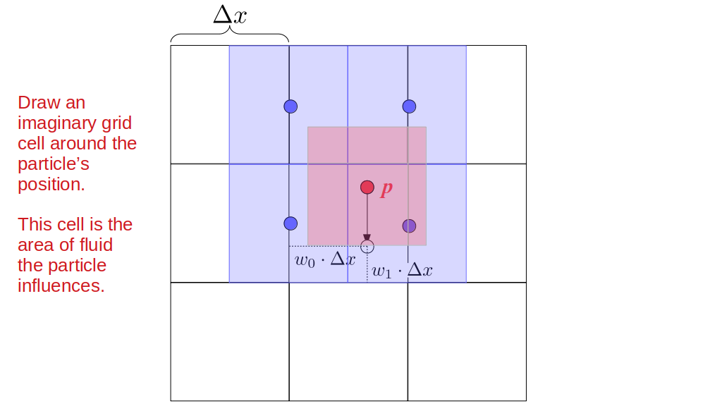
What is the area of overlap between the particle's imaginary grid cell and each of the velocity components' grid cells?

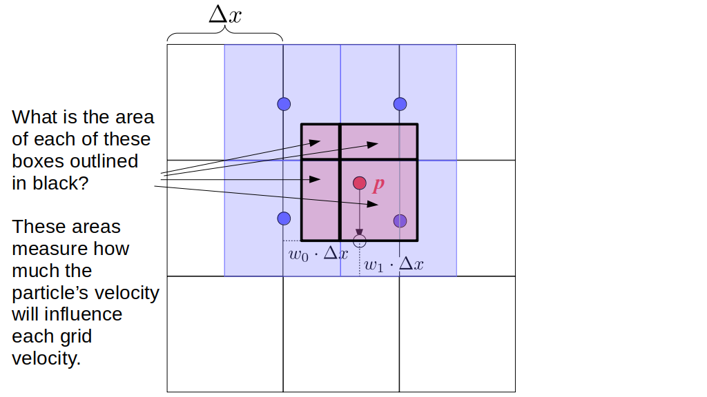
To help us calculate these areas, let's define a few horizontal vectors:

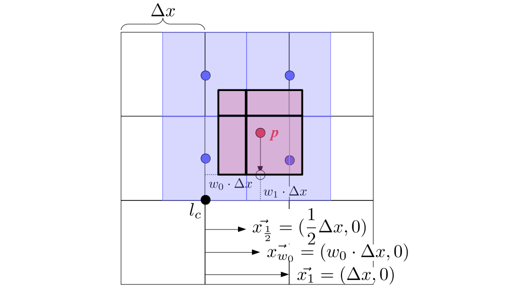
And a few vertical ones:

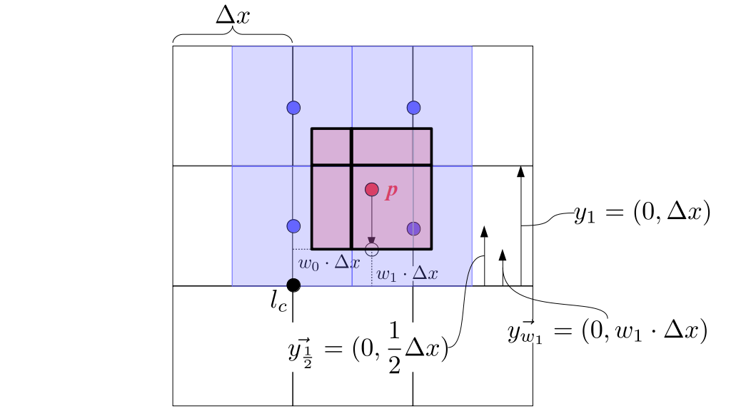
Note that by the definition of the downward shift process, we can reach the particle's position by starting at the lower corner of the grid cell into which we shifted, going right by w₀ · Δx, going up by w₁ · Δx, and then going up by ½Δx:

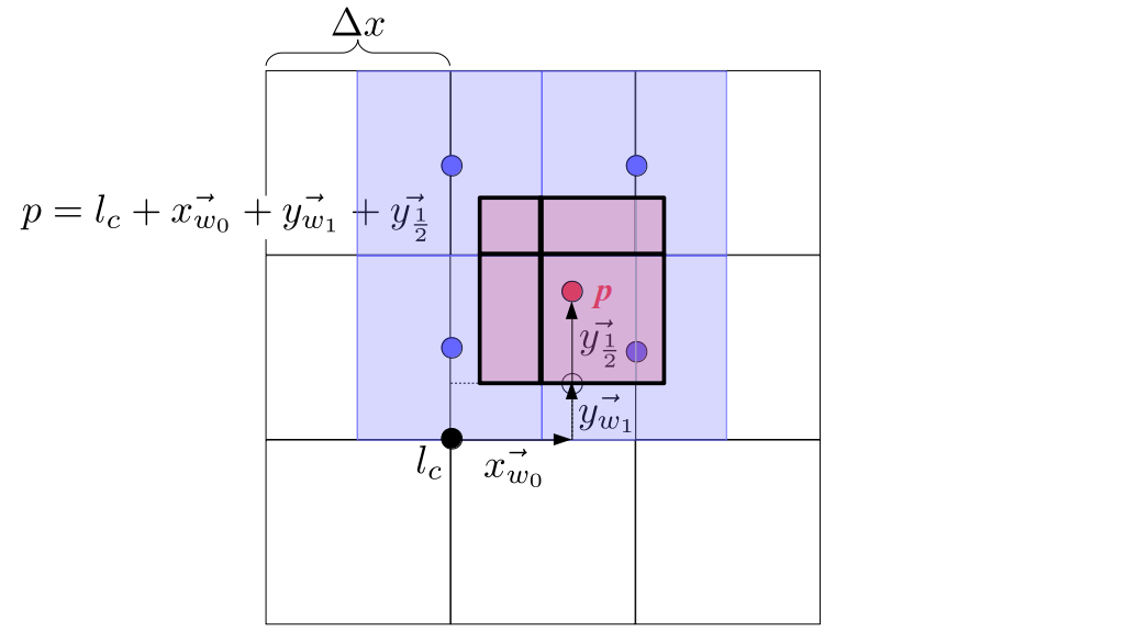
Then, you can reach the lower left corner of the particle-centered imaginary grid cell by going down by ½Δx and then left by ½Δx:

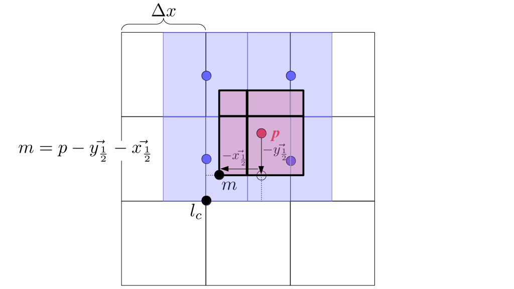
Then you can reach the other corners by going up by Δx:

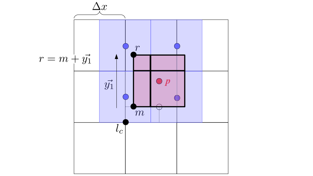
Right by Δx:

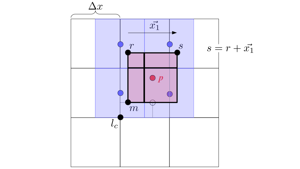
And right from the lower left corner by Δx:

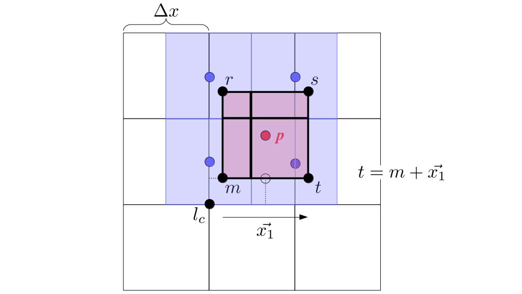
We can reach the point at the top of this grid cell and halfway across by starting at the lower left corner of the grid cell, going right by ½Δx and up by Δx:

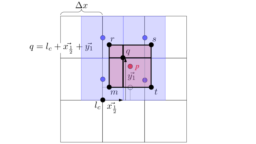
Doing a little vector algebra, e.g., subtracting that last point by the top left corner of the particle-centered imaginary grid cell, we see that the rectangle whose diagonally opposite corners are those two points is a (1 - w₀) ✕ w₁ rectangle:

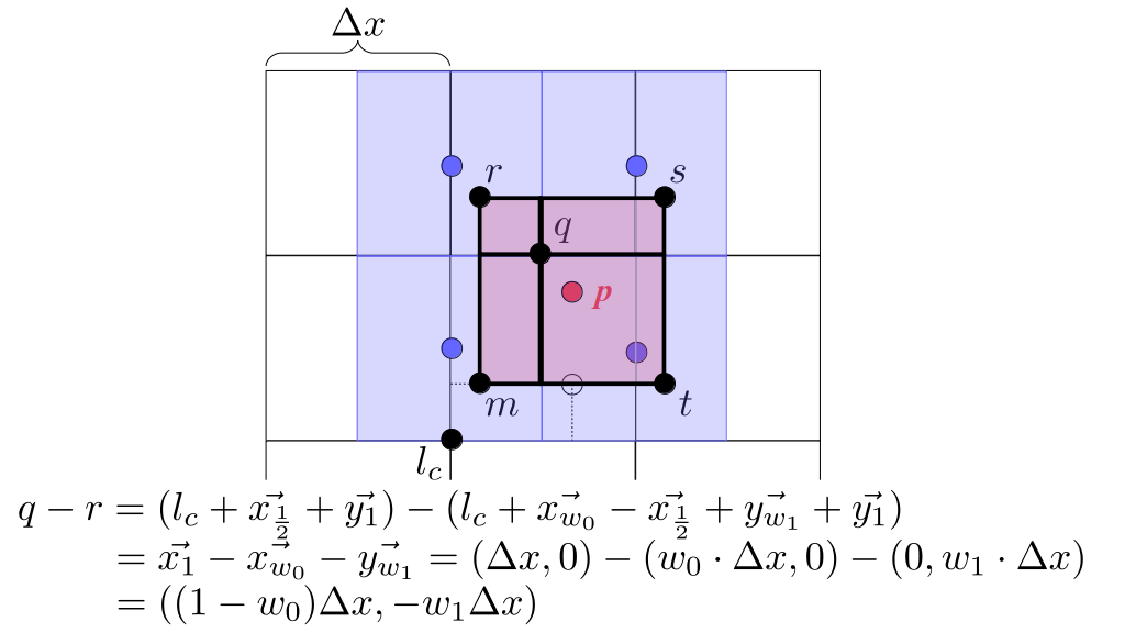
So its area is (1 - w₀)w₁(Δx)²:

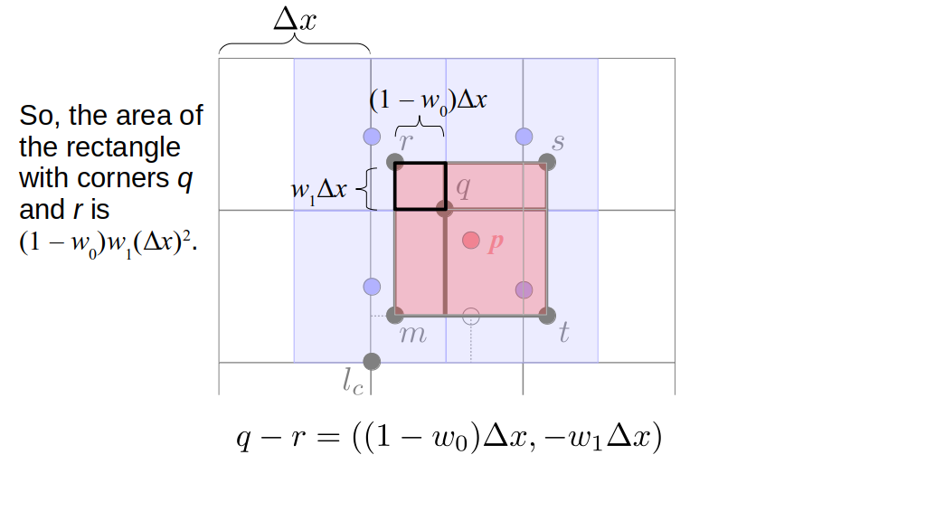
Similar vector algebra will reveal that the area of the top right rectangle of overlap is w₀w₁(Δx)², the area of the bottom left rectangle of overlap is (1 - w₀)(1 - w₁)(Δx)², and the area of the bottom right rectangle of overlap is w₀(1 - w₁)(Δx)²:

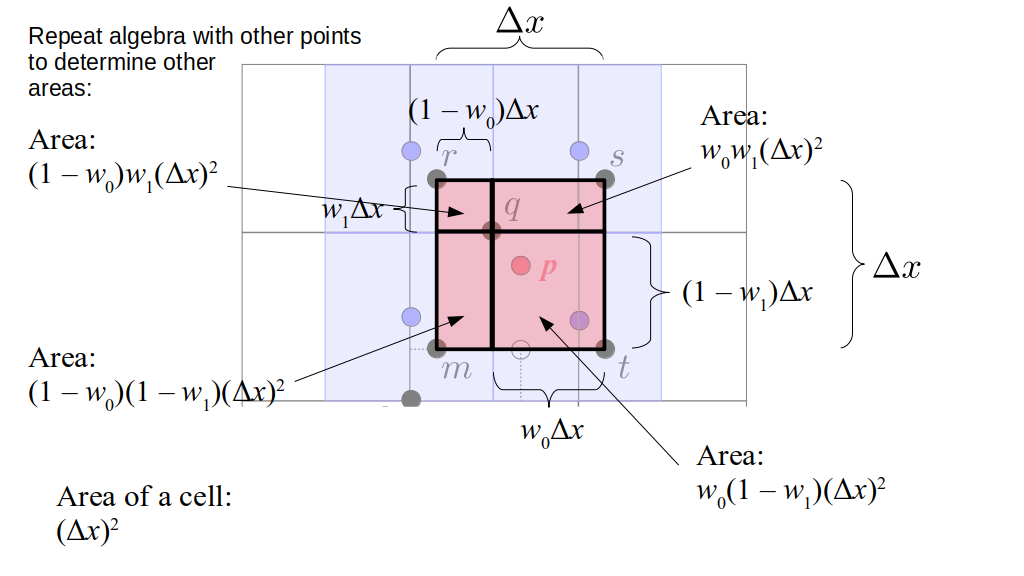
The area of a grid cell is (Δx)², so we could say the areas of these rectangles are the fractions (1 - w₀)(1 - w₁), w₀(1 - w₁), (1 - w₀)w₁, and w₀w₁ of a grid cell. Remember where we've seen these before! These are the coefficients we multiply the particle's horizontal velocity by to get the particle's contributions to the four velocities it influences!

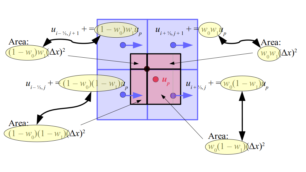
So, you can think of it like this:

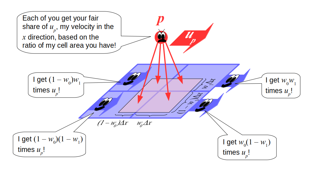
That is, the particle exerts influence onto its neighboring velocity components. The amount of influence it exerts on each velocity component is proportional to how much its imaginary grid cell overlaps each velocity component's imaginary grid cell! This is called area-weighted interpolation and is used in a variety of related operations in computational fluid dynamics and computer graphics. For example, on page 15 (page 18 of the PDF) of a report by Francis H. Harlow (1962), a related "velocity weighting procedure" of mapping from the grid velocities to a particle's velocity is described. Similarly, Figure 3 of a key paper by Foster and Metaxas (1996) that introduced computational fluid dynamics to computer graphics illustrates an area-weighted interpolation scheme for mapping the velocity of a "marker particle" (a slightly different concept than our actual fluid particles) based on grid velocities.

Note that for all particles we use to model a fluid, we would repeat this process: for each particle, splat its velocities onto the grid via this process. FLIP fluid simulation algorithms use a variety of approaches for finding these neighboring grid cells for splatting, or transferring, velocities from particles to the grid. In this case, we are using our area-weighted interpolation approach for the particle-to-grid transfer. See the paper by Ding et al. (2019) for a more detailed introduction to the trade-offs around velocity transfers in PIC/FLIP algorithms.

Splatting Particle Velocities onto the Grid in 3D

The figures below show how we will illustrate the three-dimensional neighborhood of grid cells around a particle. We'll spread adjacent grid cells in a slice of cells apart for easier viewing:

We'll also spread the z direction slices of grid cells out from each other so it's easier to see things without overlap.

Splatting in 3D works the same as 2D, with a few small changes to account for the extra dimension. We still shift half a grid cell width from the particle's position, but we do it now in two coordinate directions instead of one. We also still splat the particle's velocity onto neighboring grid velocities, but now we will have eight grid velocity components to update instead of just four.

Here is the whole 3D splatting procedure, in three parts. The first part is the update of the x-direction grid velocity components:

• Shift from the particle's position, (x, y, z) by -Δx/2 in the y and z directions to the point (x, y - Δx/2, z - Δx/2).
• Calculate the barycentric weights of that shifted position relative to the cell containing that point. If you shifted onto a cell boundary, assume you're in the cell with the higher index in the relevant coordinate direction(s).
• Splat the particle's u velocity (the x component of its velocity) onto the u velocity components of the grid cell containing this shifted position. Also splat the particle's u velocity component onto the u velocity components of the grid cell in front of, the grid cell above, and the grid cell diagonally in front of and above, that grid cell containing the shifted position.

The second part of the 3D splatting algorithm is the update of grid velocities in the y direction:

• Shift from the particle's position, (x, y, z), by -Δx/2 in the x and z directions to the point (x - Δx/2, y, z - Δx/2).
• Calculate the barycentric weights of that shifted position relative to the cell containing that point. If you shifted onto a cell boundary, assume you're in the cell with the higher index in the relevant coordinate direction(s).
• Splat the particle's v velocity (the y component of its velocity) onto the v velocity components of the grid cell containing this shifted position. Also splat the particle's v velocity component onto the v velocity components of the grid cell to the right of, in front of, and diagonally to the right and in front of, that grid cell containing the shifted position.

The third part of the 3D splatting algorithm is the update of grid velocities in the z direction:

• Shift from the particle's position, (x, y, z), by -Δx/2 in the x and y directions to the point (x - Δx/2, y - Δx/2, z).
• Calculate the barycentric weights of that shifted position relative to the cell containing that point. If you shifted onto a cell boundary, assume you're in the cell with the higher index in the relevant coordinate direction(s).
• Splat the particle's w velocity (the z component of its velocity) onto the w velocity components of the grid cell containing this shifted position. Also splat the particle's w velocity component onto the w velocity components of the grid cell to right of, above, and diagonally above and to the right of, that grid cell containing the shifted position.

As with the 2D splatting algorithm, all of these parts of the 3D splatting algorithm are done once for each particle in the entire simulation, in each time step.

Now, implementing this algorithm can actually be done in a very small amount of code, but understanding how it works is complicated by the fact that, in each of the three parts of the algorithm above, the shift step can end up in different grid cells depending on where exactly the particle was located in its original cell. Let's look at this carefully.

For the first part of the splatting algorithm, the negative half-grid-cell-width shift in the y and z directions will land you in one of four possible grid cells, depending on in which quadrant of its current grid cell the particle is located:

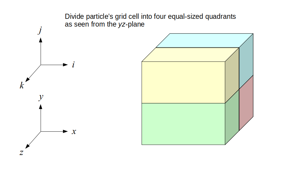
Case 1: shift to the cell diagonally below and back:

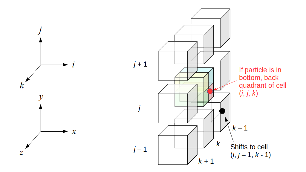
In that case, the velocity components we update are:

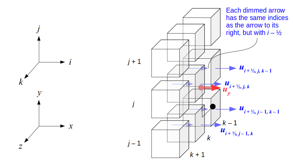
And here's how we update them:

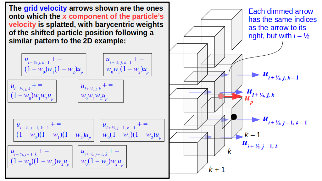
Case 2: shift to the cell below:

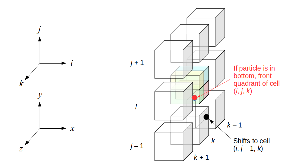
In that case, the velocity components we update are:

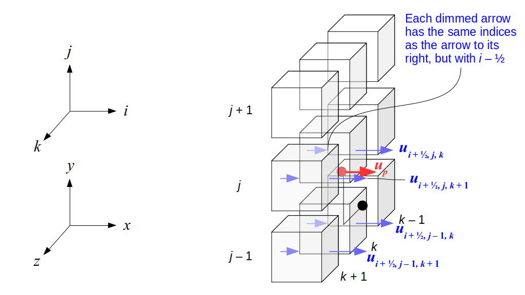
And here's how we update them:

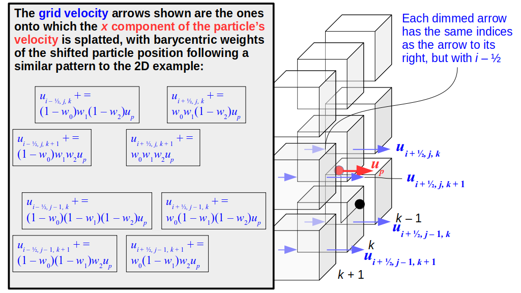
Case 3: shift to the cell behind the particle's cell:

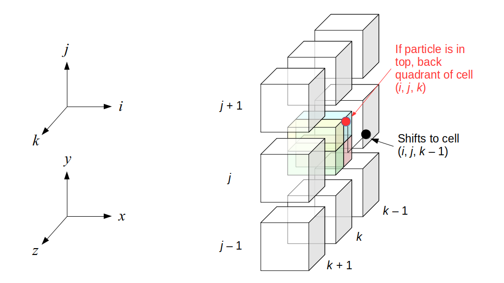
In that case, the velocity components we update are:

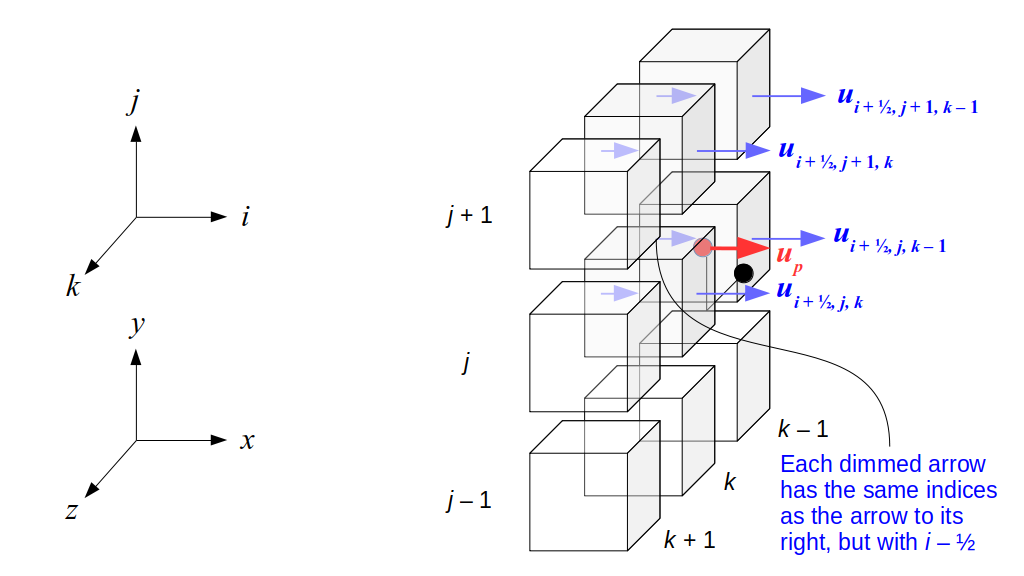
And here's how we update them:

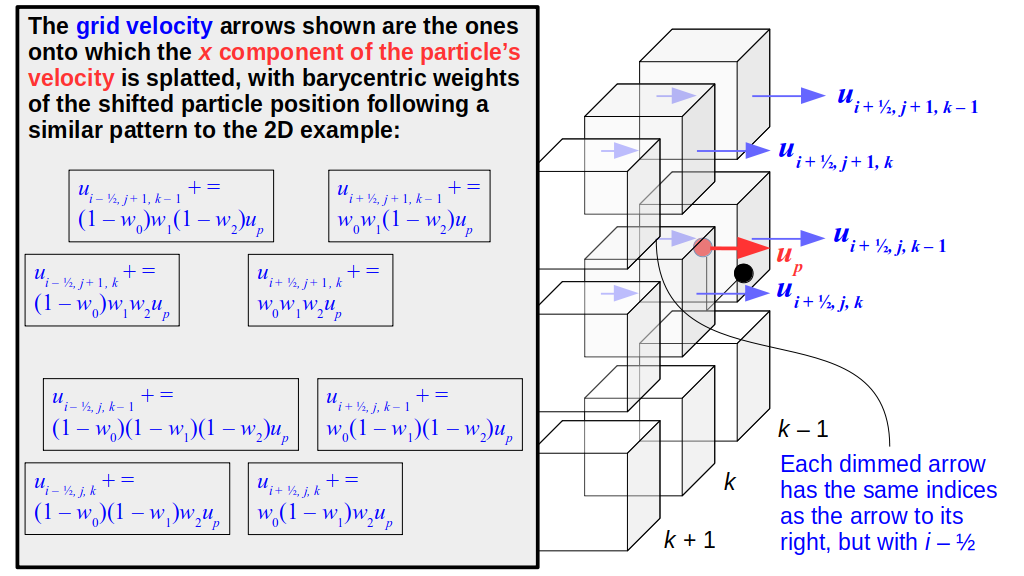
Case 4: stay in the same grid cell after the shift:

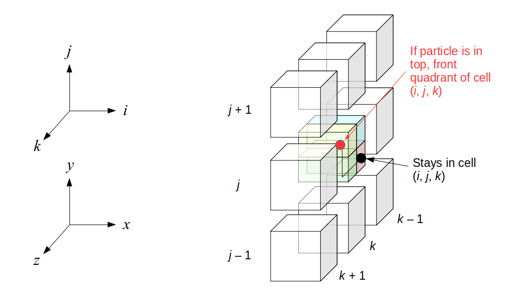
In that case, the velocity components we update are:

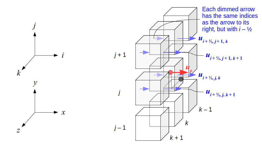
And here's how we update them:

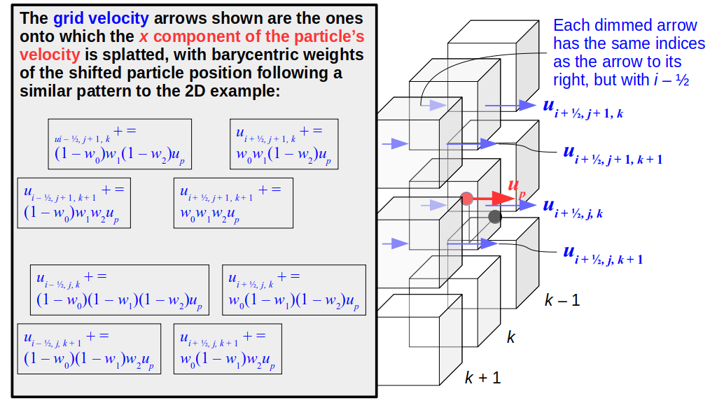
For the second part of the splatting algorithm, the negative shift in the x and z directions will land you in one of four possible grid cells, depending on in which quadrant of its current grid cell the particle is located:

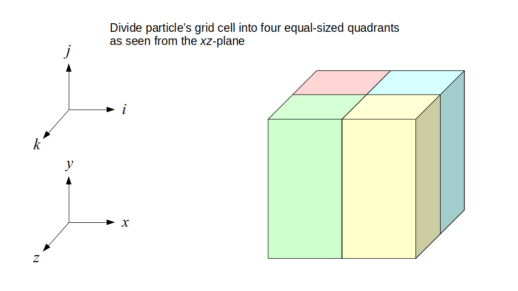
Case 1: shift to the cell diagonally left and back:

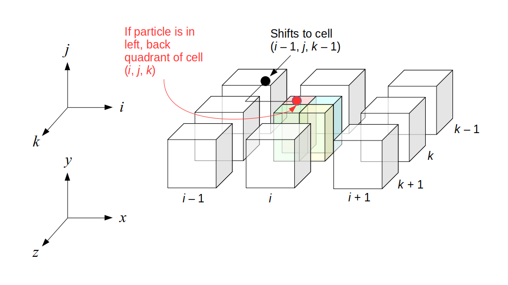
In that case, the velocity components we update are:

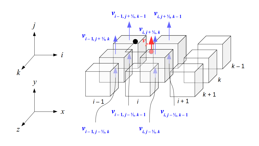
And here's how we update them:

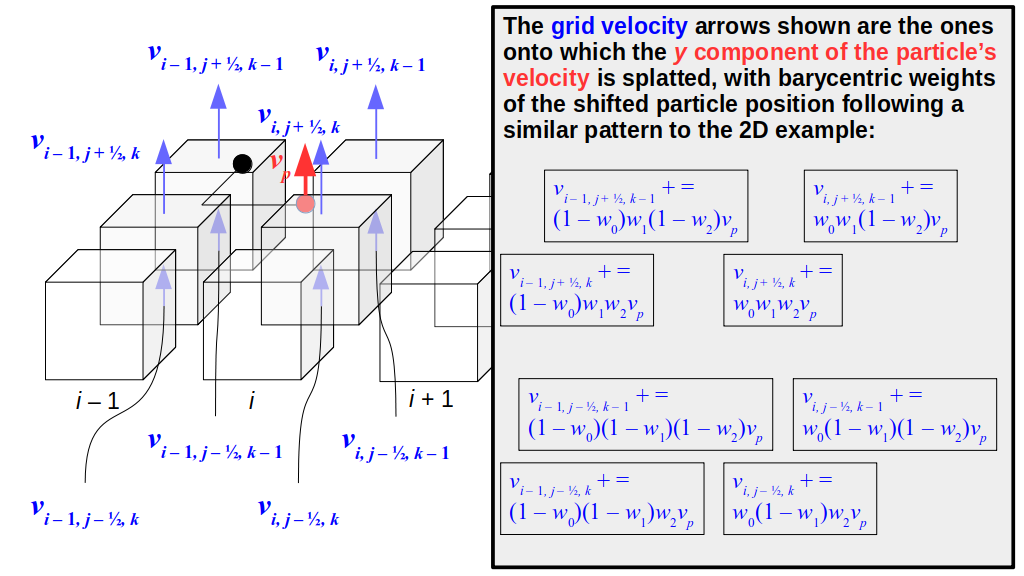
Case 2: shift to the cell to the left:

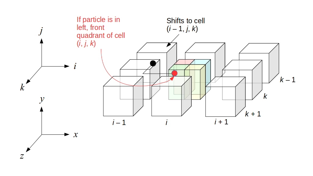
In that case, the velocity components we update are:

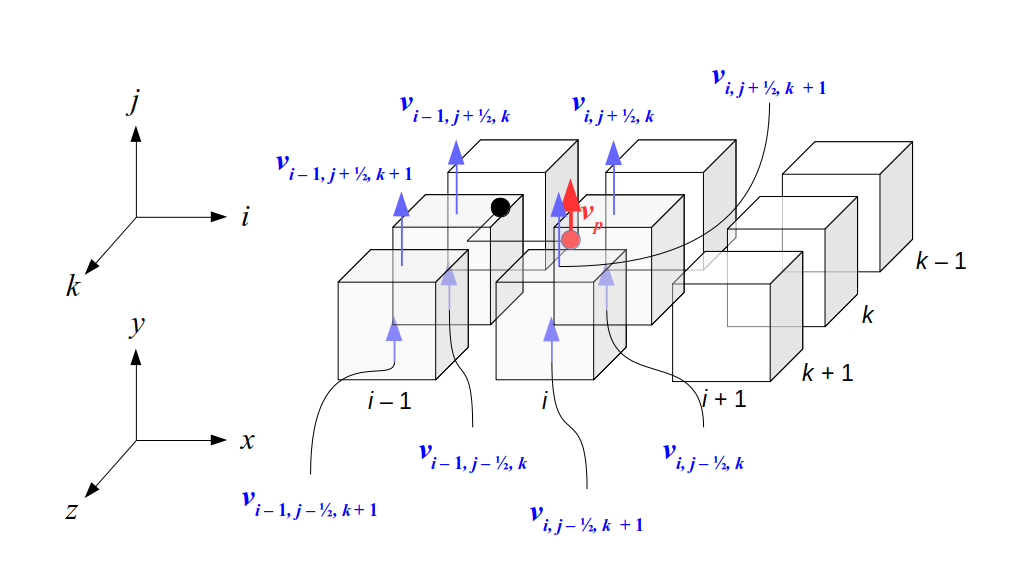
And here's how we update them:

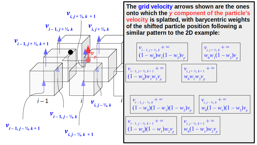
Case 3: shift to the cell behind the particle's cell:

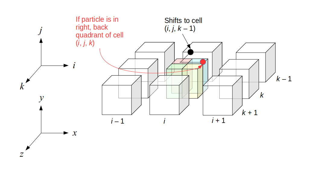
In that case, the velocity components we update are:

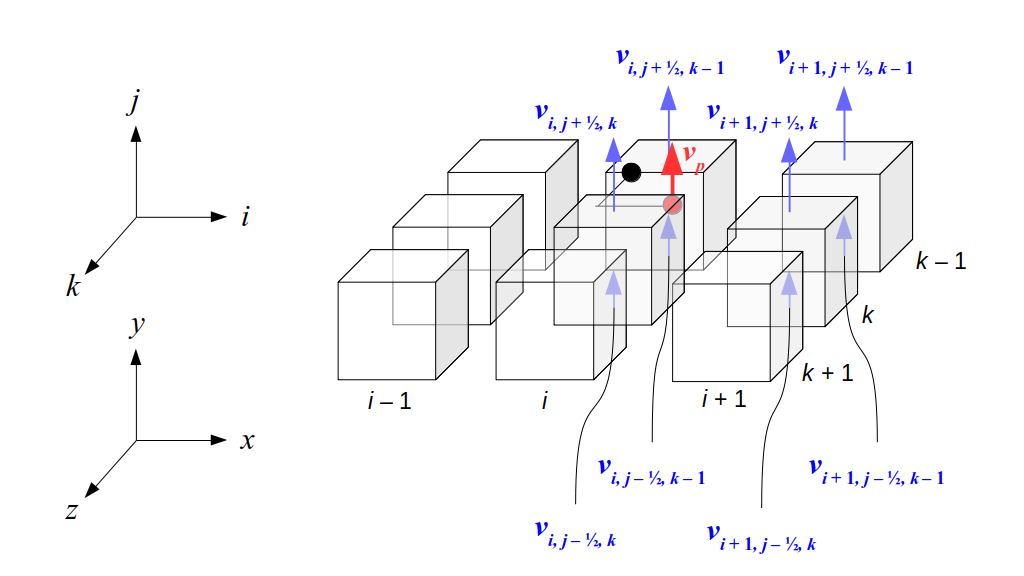
And here's how we update them:

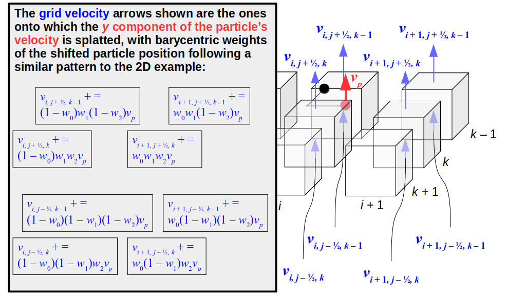
Case 4: stay in the same grid cell after the shift:

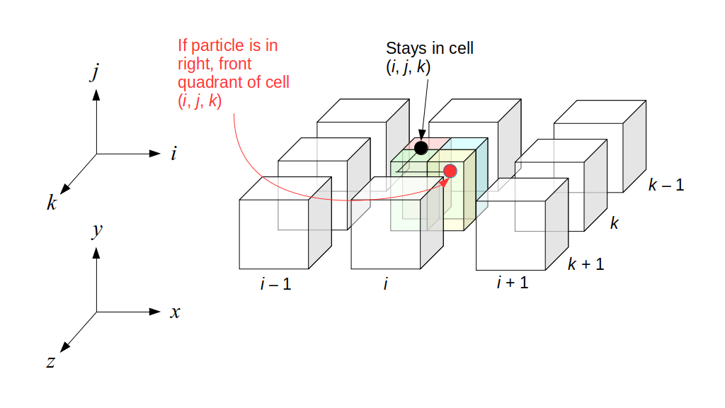
In that case, the velocity components we update are:

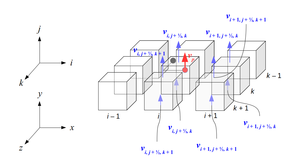
And here's how we update them:

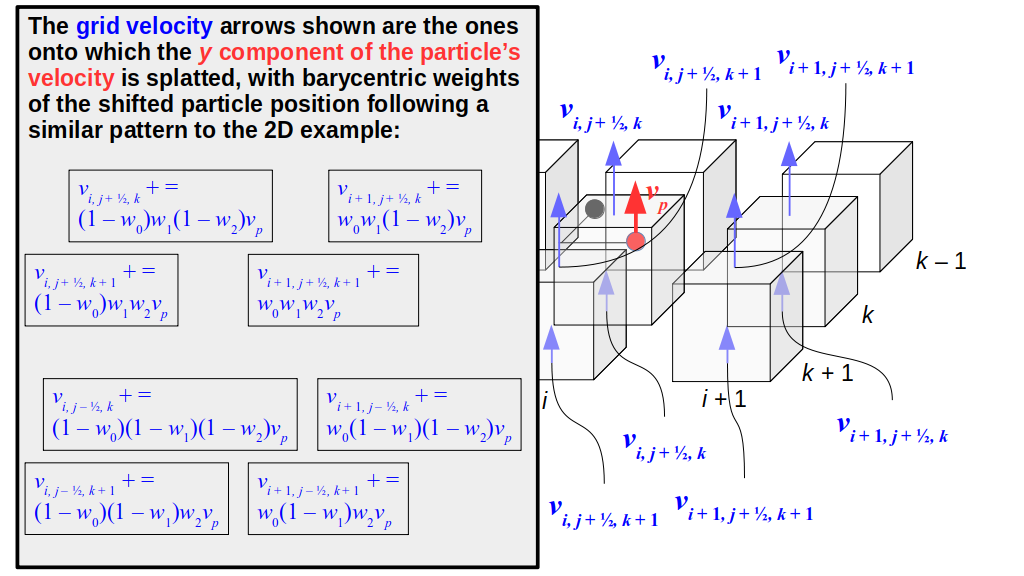
For the third part of the splatting algorithm, the negative shift in the x and y directions will land you in one of four possible grid cells, depending on in which quadrant of its current grid cell the particle is located:

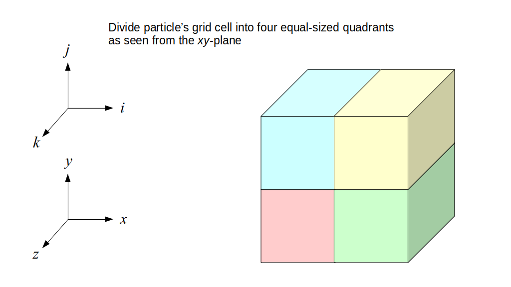
Case 1: shift to the cell diagonally left and down:

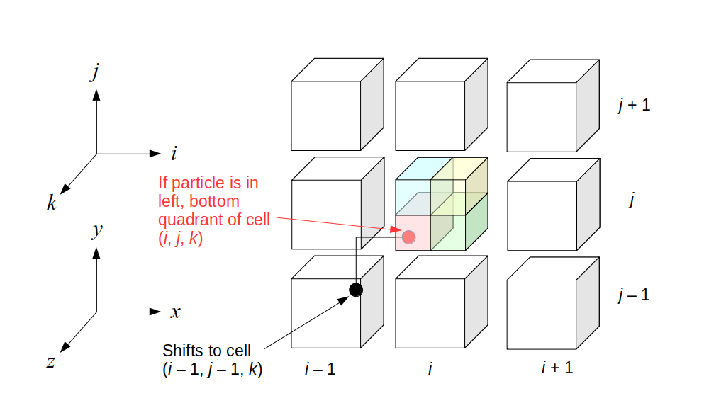
In that case, the velocity components we update are:

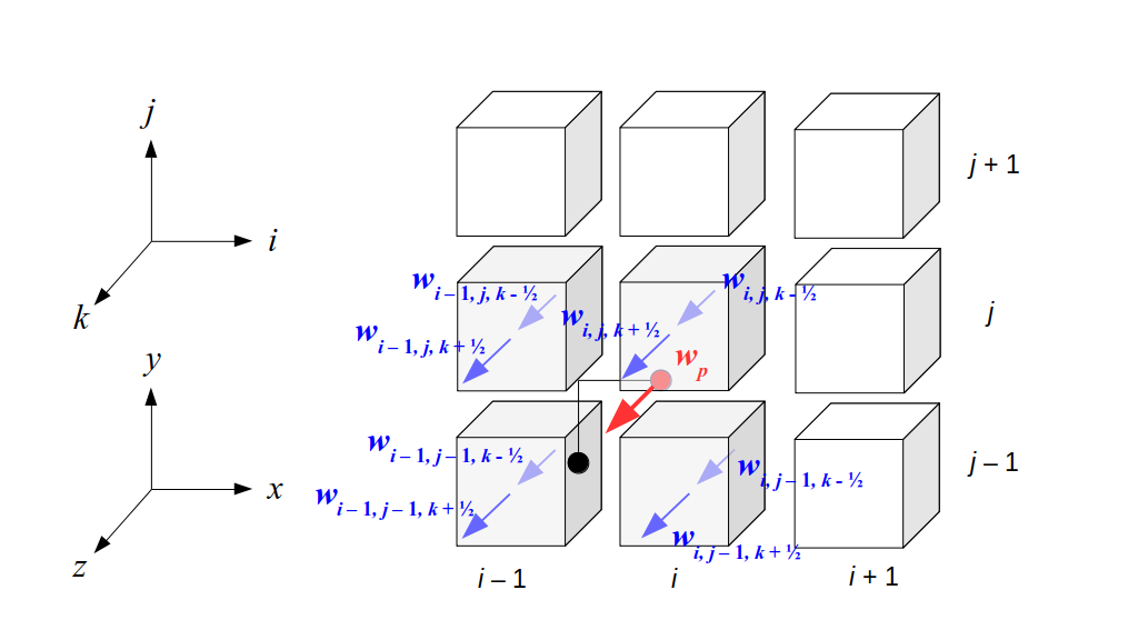
And here's how we update them:

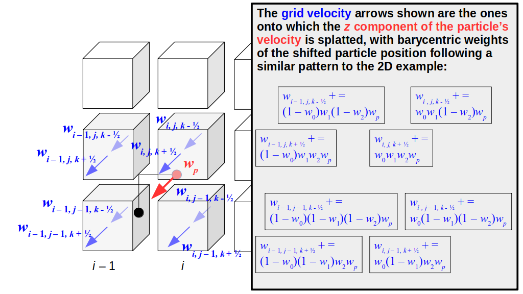
Case 2: shift to the cell to the left:

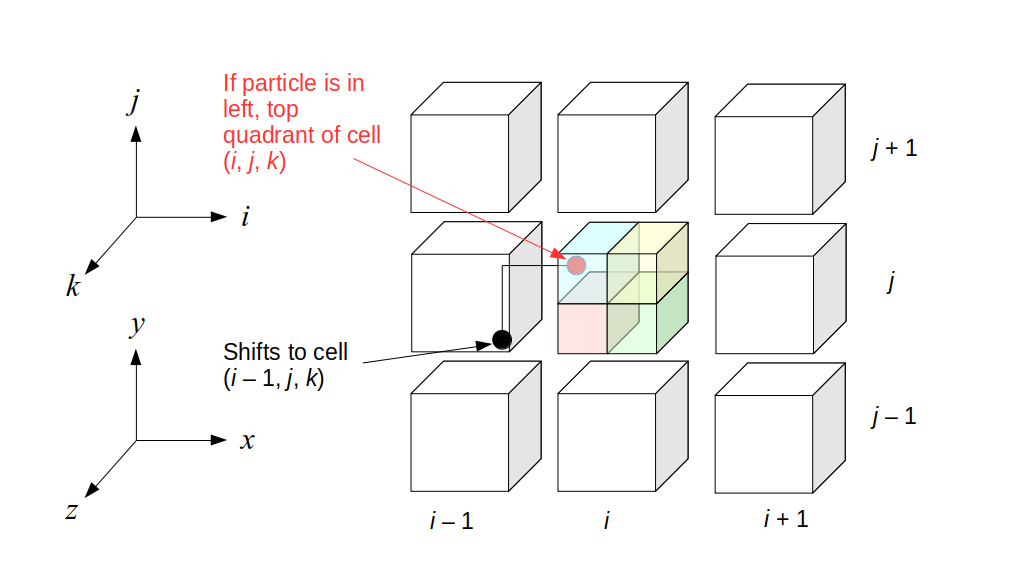
In that case, the velocity components we update are:

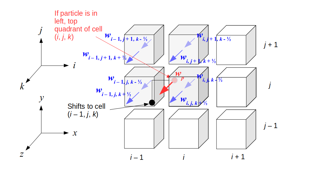
And here's how we update them:

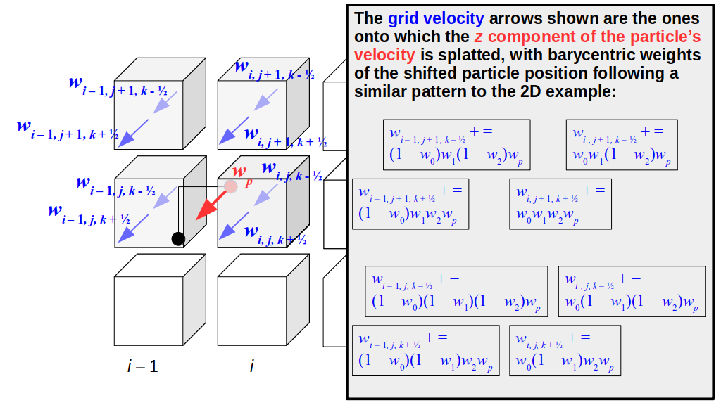
Case 3: shift to the cell below the particle's cell:

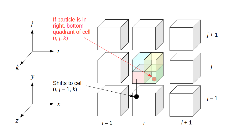
In that case, the velocity components we update are:

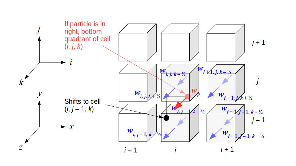
And here's how we update them:

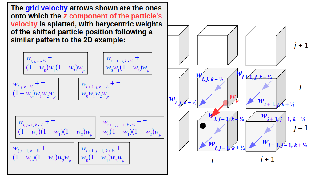
Case 4: stay in the same grid cell after the shift:

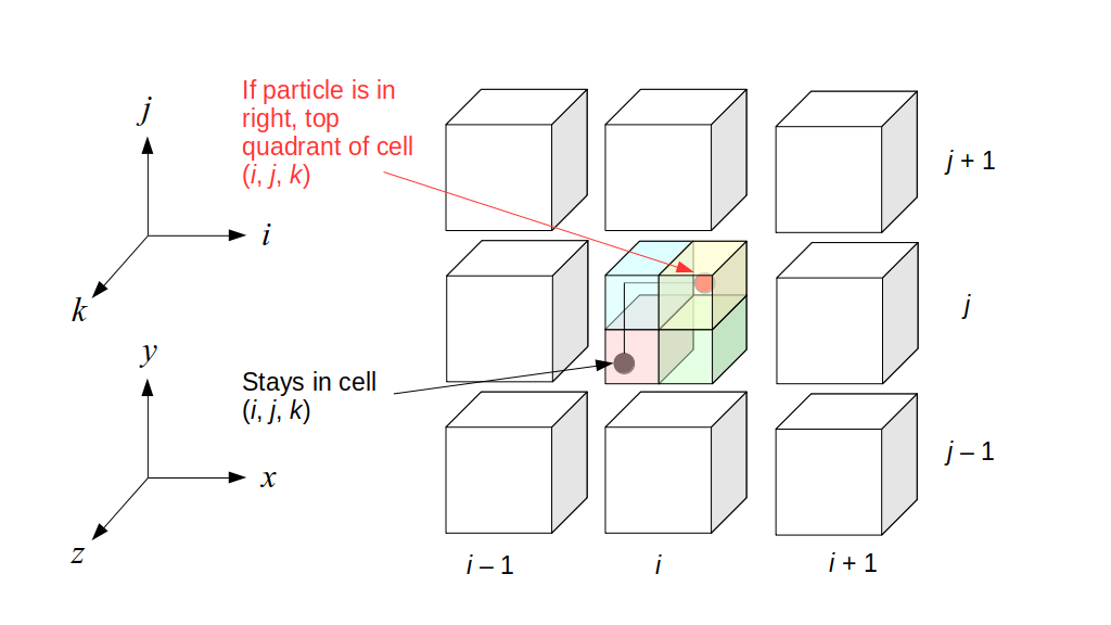
In that case, the velocity components we update are:

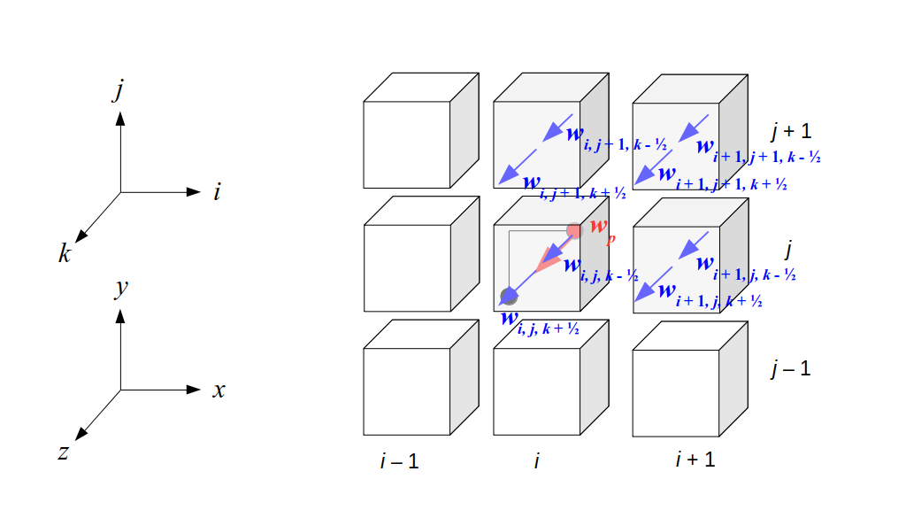
And here's how we update them:

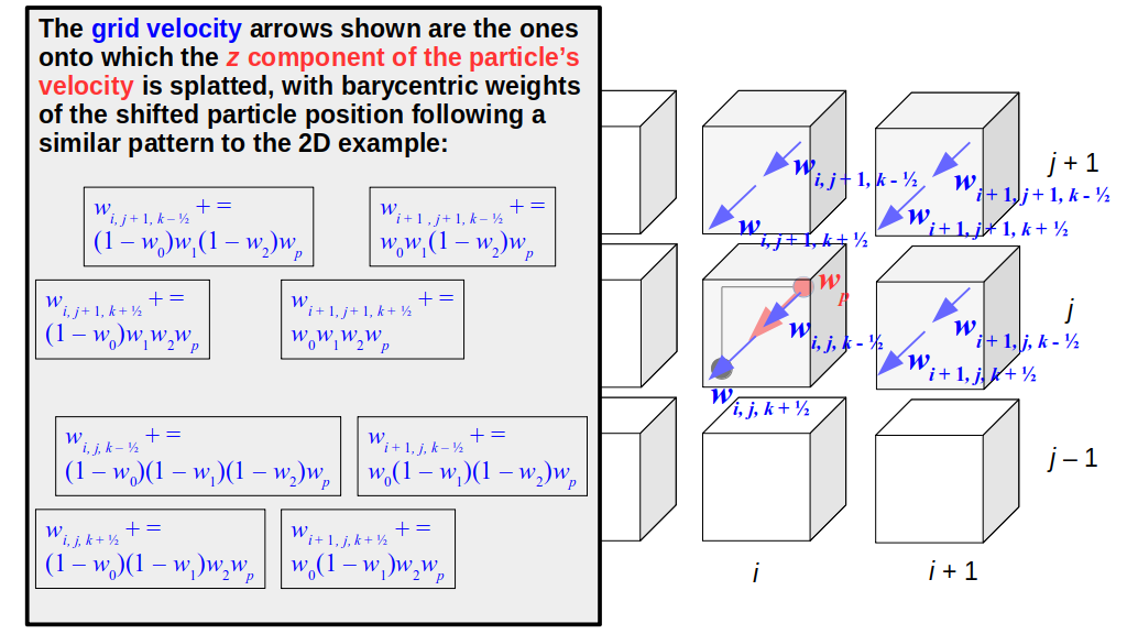
Note that all this gymnastics with shifting and indexing is doing the exact same thing we did in the 2D case: the shift finds the lower corner of the imaginary grid cell centered at the particle, and then we use the weighted volumes of overlap between that cell and the imaginary grid cell centered around each of the neighboring grid velocity components.

Interestingly, in the diagrams above, if we let (i_shifted, j_shifted, k_shifted) denote the grid cell you shifted into, then after the shift in the y and z directions, we always update the u velocities on either side of these four grid cells:

• (i_shifted, j_shifted, k_shifted)
• (i_shifted, j_shifted + 1, k_shifted)
• (i_shifted, j_shifted, k_shifted + 1)
• (i_shifted, j_shifted + 1, k_shifted + 1)

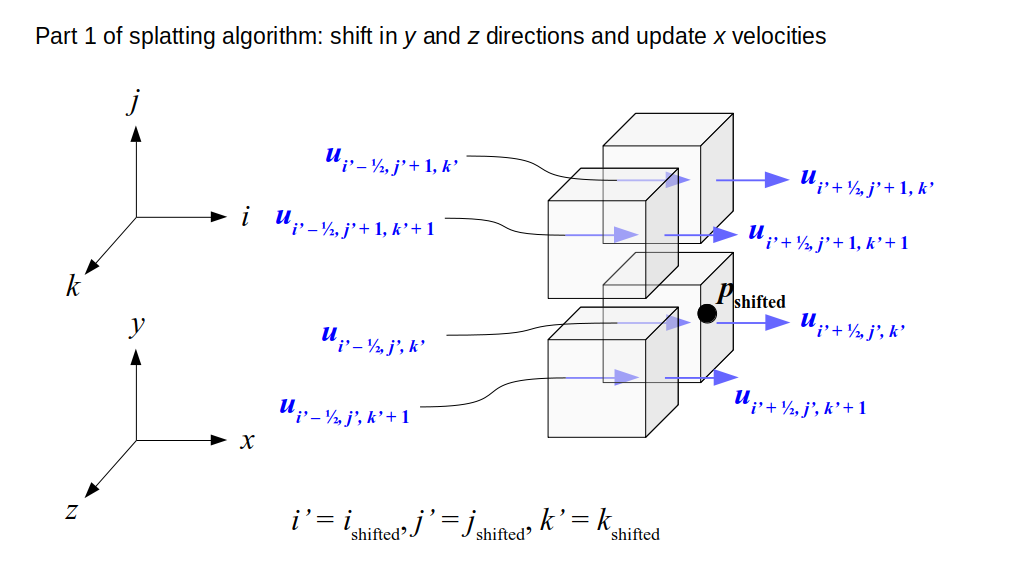
Similarly, after the shift in the x and z directions, we always update the v velocities on either side of these four grid cells:

• (i_shifted, j_shifted, k_shifted)
• (i_shifted + 1, j_shifted, k_shifted)
• (i_shifted, j_shifted, k_shifted + 1)
• (i_shifted + 1, j_shifted, k_shifted + 1)

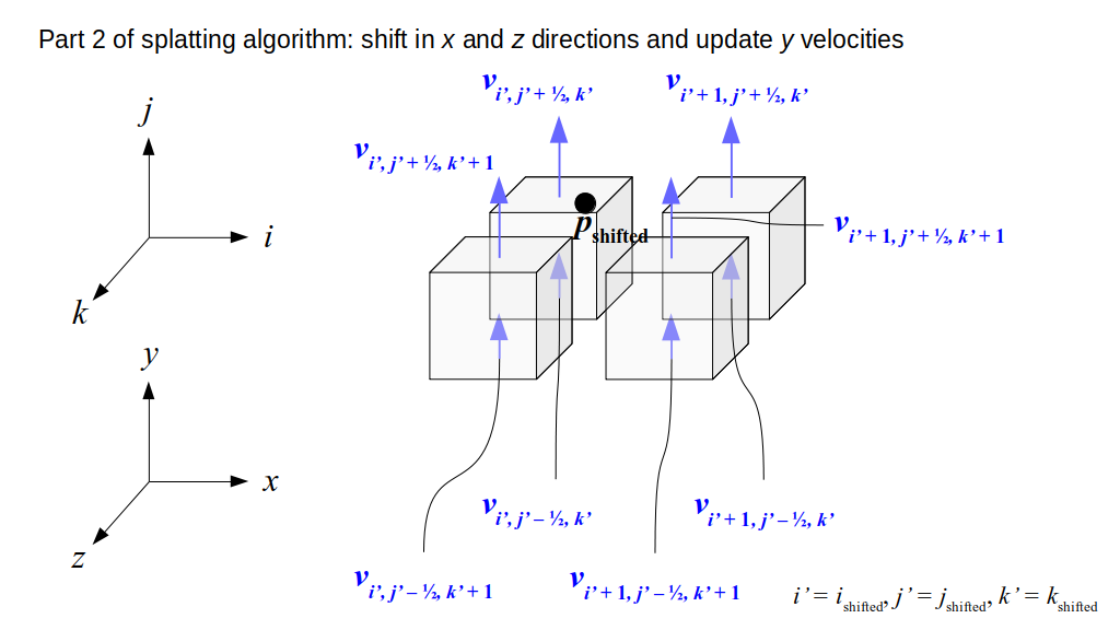
And after the shift in the y and z directions, we always update the w velocities on either side of these four grid cells:

• (i_shifted, j_shifted, k_shifted)
• (i_shifted + 1, j_shifted, k_shifted)
• (i_shifted, j_shifted + 1, k_shifted)
• (i_shifted + 1, j_shifted + 1, k_shifted)

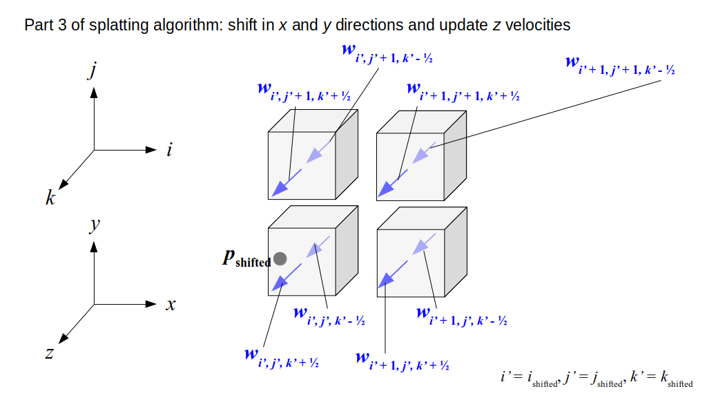
Now recall that, our indexing scheme getting rid of the ½s in our indices makes the -½s disappear and the +½s become +1s:

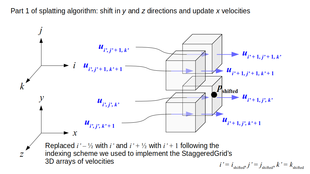
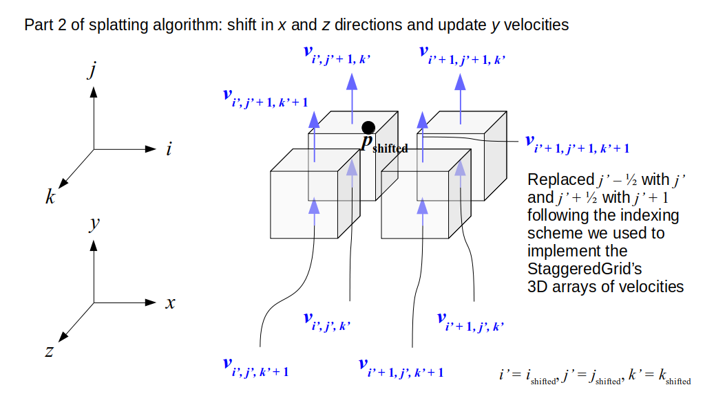
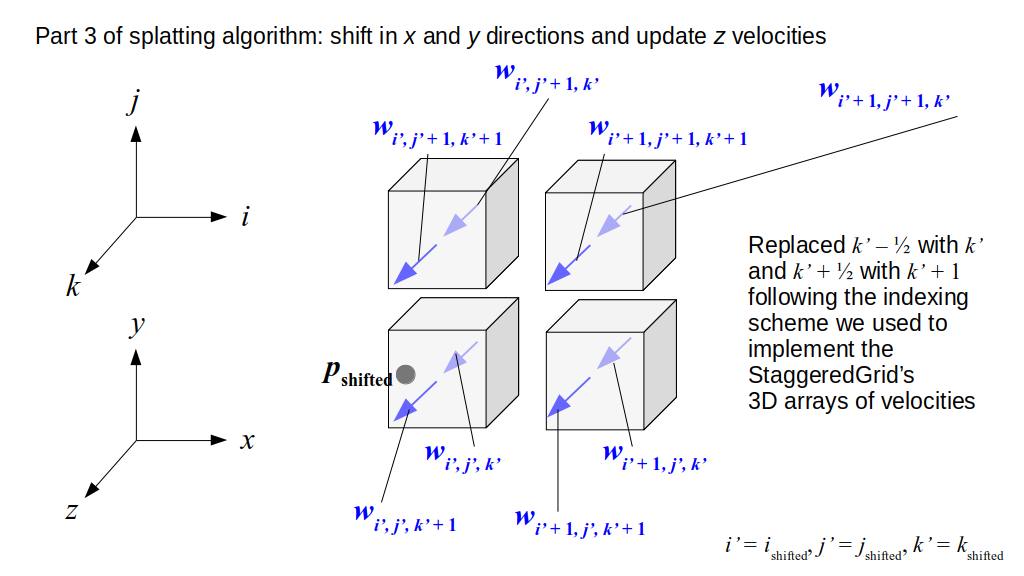
Let's list all the velocities we end up updating that are shown in the diagrams above with the indexing scheme we use in our code for the staggered grid's 3D arrays of velocities. The velocities we end up updating in our staggered grid's 3D arrays of velocities, based on the u velocity-update list above, are (note that i_shifted can be i or i - 1, j_shifted can be j or j - 1, and k_shifted can be k or k - 1 as in the diagrams above depending on where the shift lands, so i_shifted + 1 would be either i or i + 1, j_shifted + 1 would be either j or j + 1, and k_shifted + 1 would be either k or k + 1):

• u(i_shifted, j_shifted, k_shifted)
• u(i_shifted + 1, j_shifted, k_shifted)
• u(i_shifted, j_shifted + 1, k_shifted)
• u(i_shifted + 1, j_shifted + 1, k_shifted)
• u(i_shifted, j_shifted, k_shifted + 1)
• u(i_shifted + 1, j_shifted, k_shifted + 1)
• u(i_shifted, j_shifted + 1, k_shifted + 1)
• u(i_shifted + 1, j_shifted + 1, k_shifted + 1)

And the velocities we end up updating in the 3D array of v velocities are:

• v(i_shifted, j_shifted, k_shifted)
• v(i_shifted, j_shifted + 1, k_shifted)
• v(i_shifted + 1, j_shifted, k_shifted)
• v(i_shifted + 1, j_shifted + 1, k_shifted)
• v(i_shifted, j_shifted, k_shifted + 1)
• v(i_shifted, j_shifted + 1, k_shifted + 1)
• v(i_shifted + 1, j_shifted, k_shifted + 1)
• v(i_shifted + 1, j_shifted + 1, k_shifted + 1)

And the velocities we end up updating in the 3D array of w velocities are:

• w(i_shifted, j_shifted, k_shifted)
• w(i_shifted, j_shifted, k_shifted + 1)
• w(i_shifted + 1, j_shifted, k_shifted)
• w(i_shifted + 1, j_shifted, k_shifted + 1)
• w(i_shifted, j_shifted + 1, k_shifted)
• w(i_shifted, j_shifted + 1, k_shifted + 1)
• w(i_shifted + 1, j_shifted + 1, k_shifted)
• w(i_shifted + 1, j_shifted + 1, k_shifted + 1)

So, we can use the same set of indices (i, j, k of the cell containing the shifted particle position, each plus 1 or not) to access every velocity component in every direction that we need to update! Putting it all together, the whole 3D splatting algorithm will work like this (as you can also see in Bargteil and Shinar's fluid.cpp file):

• Let p.pos = (x, y, z) denote the position of the particle p at the current time step.
• Part 1: Splat horizontal velocity of particle onto grid:
  • Let p_shifted = (x, y - Δx / 2, z - Δx / 2).
  • Let (i, j, k) be the indices of the grid cell containing p_shifted.
  • Let (w₀, w₁, w₂) be the barycentric weights of p_shifted in grid cell (i, j, k).
  • splat(u_p, w₀, w₁, w₂, i, j, k, u_grid): This splats the particle's horizontal velocity, u_p, whose shifted position lies in cell (i, j, k) with barycentric weights (w₀, w₁, w₂), onto the relevant velocities in the 3D array, u_grid, of horizontal velocity components on the grid.
• Part 2: Splat vertical velocity of particle onto grid:
  • Let p_shifted = (x - Δx / 2, y, z - Δx / 2).
  • Let (i, j, k) be the indices of the grid cell containing p_shifted.
  • Let (w₀, w₁, w₂) be the barycentric weights of p_shifted in grid cell (i, j, k).
  • splat(v_p, w₀, w₁, w₂, i, j, k, v_grid): This splats the particle's vertical velocity, v_p, whose shifted position lies in cell (i, j, k) with barycentric weights (w₀, w₁, w₂), onto the relevant velocities in the 3D array, v_grid, of vertical velocity components on the grid.
• Part 3: Splat depth (z direction) velocity of particle onto grid:
  • Let p_shifted = (x - Δx / 2, y - Δx / 2, z).
  • Let (i, j, k) be the indices of the grid cell containing p_shifted.
  • Let (w₀, w₁, w₂) be the barycentric weights of p_shifted in grid cell (i, j, k).
  • splat(w_p, w₀, w₁, w₂, i, j, k, w_grid): This splats the particle's depth velocity, w_p, whose shifted position lies in cell (i, j, k) with barycentric weights (w₀, w₁, w₂), onto the relevant velocities in the 3D array, w_grid, of depth velocity components on the grid.

Where the splat function is:

splat(vel_p, w₀, w₁, w₂, i, j, k, vel_grid):

• vel_grid(i, j, k) += (1 - w₀) · (1 - w₁) · (1 - w₂) · vel_p
• vel_grid(i + 1, j, k) += w₀ · (1 - w₁) · (1 - w₂) · vel_p
• vel_grid(i, j + 1, k) += (1 - w₀) · w₁ · (1 - w₂) · vel_p
• vel_grid(i + 1, j + 1, k) += w₀ · w₁ · (1 - w₂) · vel_p
• vel_grid(i, j, k + 1) += (1 - w₀) · (1 - w₁) · w₂ · vel_p
• vel_grid(i + 1, j, k + 1) += w₀ · (1 - w₁) · w₂ · vel_p
• vel_grid(i, j + 1, k + 1) += (1 - w₀) · w₁ · w₂ · vel_p
• vel_grid(i + 1, j + 1, k + 1) += w₀ · w₁ · w₂ · vel_p

Note that (i, j, k) here are the indices of the cell containing the shifted particle position, which may be different for each of the shifts we do in the three different parts of the 3D splatting algorithm.

Anyway, because of our indexing scheme, all of these different cases of shifting in different coordinate directions and splatting onto neighboring grid cell velocities just works, by calling this one fixed splat function three times with different inputs!

But there's a problem!

Normalizing Splatted Velocities

What would happen if we had a ton of particles influencing certain grid velocities?

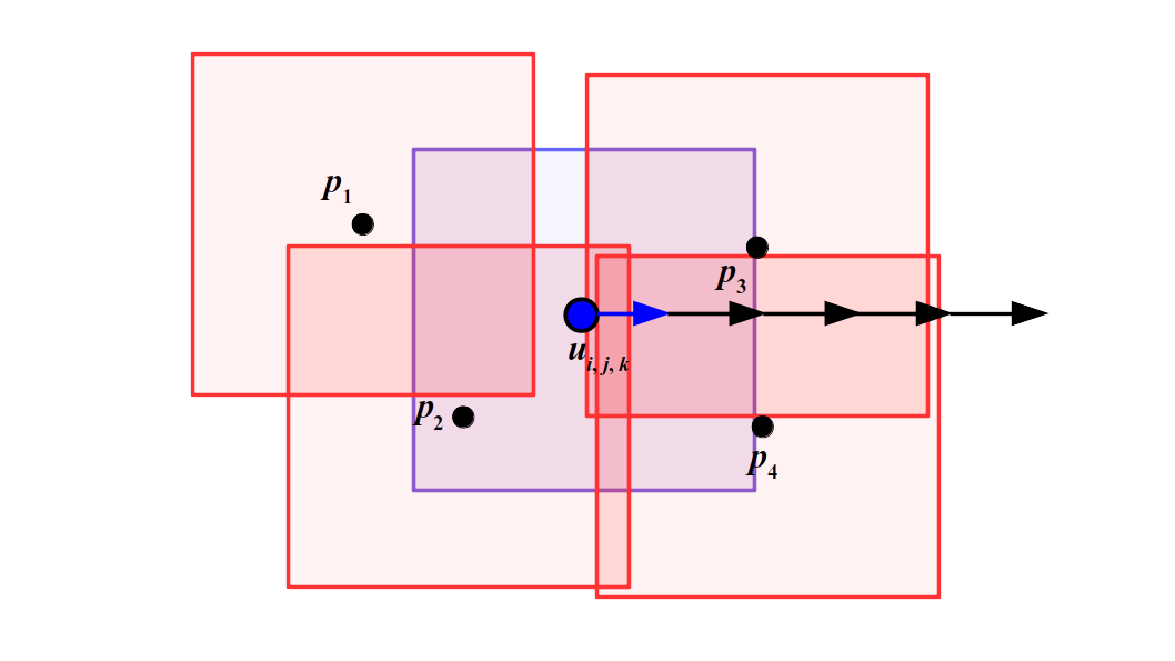
Basically, we would keep adding, and adding, and adding, and adding more and more weighted particle velocities to those grid velocities. If you had a hundred million particles all moving at 6 m/s in a direction parallel to a grid velocity and having their imaginary cells overlapping half the volume of a grid velocity's imaginary cell, your fluid velocity would exceed the speed of light (which is just under 300 million m/s)! Sorry, but your fluid is not moving that fast! Okay that's an extreme example, but the point is, we don't want fluid velocities to be huge just because there are a lot of particles near them. So, we need to normalize the value of each grid velocity component after splatting, to have it be a sort of average velocity of all particle velocities splatted onto it, rather than just a sum of those splatted particle velocities.

One approach, taken by the code associated with Bargteil and Shinar's SIGGRAPH course, is to keep adding up the volumes of overlap between the imaginary grid cell centered on each grid velocity component and the imaginary grid cell centered on each particle. That is, each time we add a particle's weighted velocity component to a grid velocity component, in parallel we sum just the weights, e.g., add up all the (1 - w₀)w₁(1 - w₂) factors for each particle's contribution to the grid velocity component u_{3 + ½, 1, 7} and so on for each grid velocity component. Then, when we're done splatting all particle velocity components onto the relevant grid velocity components, we divide each grid velocity component by that corresponding sum of all weights (volumes of overlap) of particle velocity contributions we added to that grid velocity component.

Let's modify our splatting algorithm above to add this normalization step for each velocity component in the grid. Let's also add an important detail, which is that all of the grid velocity values and all of these weight/volume sums need to be zeroed out at the beginning of our splatting algorithm (new steps are in bold):

• Let p.pos = (x, y, z) denote the position of the particle p at the current time step.
• Set every single value in all of the 3D arrays of grid velocities, u_grid, v_grid, and w_grid, to zero.
• As part of the staggered grid, just as we do with the 3D arrays u_grid, v_grid, and w_grid, store three additional 3D arrays, f_u, f_v, and f_w. Set all values in these arrays to zero as well.
• Part 1: Splat horizontal velocity of particle onto grid:
  • Let p_shifted = (x, y - Δx / 2, z - Δx / 2).
  • Let (i, j, k) be the indices of the grid cell containing p_shifted.
  • Let (w₀, w₁, w₂) be the barycentric weights of p_shifted in grid cell (i, j, k).
  • splat(u_p, w₀, w₁, w₂, i, j, k, u_grid, f_u): This splats the particle's horizontal velocity, u_p, whose shifted position lies in cell (i, j, k) with barycentric weights (w₀, w₁, w₂), onto the relevant velocities in the 3D array, u_grid, of horizontal velocity components on the grid. Also, this function will accumulate the barycentric weight products (overlap volumes) of all particle contributions to each horizontal grid velocity.
  • For each (i, j, k), divide u(i, j, k) by f_u(i, j, k).
• Part 2: Splat vertical velocity of particle onto grid:
  • Let p_shifted = (x - Δx / 2, y, z - Δx / 2).
  • Let (i, j, k) be the indices of the grid cell containing p_shifted.
  • Let (w₀, w₁, w₂) be the barycentric weights of p_shifted in grid cell (i, j, k).
  • splat(v_p, w₀, w₁, w₂, i, j, k, v_grid, f_v): This splats the particle's vertical velocity, v_p, whose shifted position lies in cell (i, j, k) with barycentric weights (w₀, w₁, w₂), onto the relevant velocities in the 3D array, v_grid, of vertical velocity components on the grid. Also, this function will accumulate the barycentric weight products (overlap volumes) of all particle contributions to each vertical grid velocity.
  • For each (i, j, k), divide v(i, j, k) by f_v(i, j, k).
• Part 3: Splat depth (z direction) velocity of particle onto grid:
  • Let p_shifted = (x - Δx / 2, y - Δx / 2, z).
  • Let (i, j, k) be the indices of the grid cell containing p_shifted.
  • Let (w₀, w₁, w₂) be the barycentric weights of p_shifted in grid cell (i, j, k).
  • splat(w_p, w₀, w₁, w₂, i, j, k, w_grid, f_w): This splats the particle's depth velocity, w_p, whose shifted position lies in cell (i, j, k) with barycentric weights (w₀, w₁, w₂), onto the relevant velocities in the 3D array, w_grid, of depth velocity components on the grid. Also, this function will accumulate the barycentric weight products (overlap volumes) of all particle contributions to each depth grid velocity.
  • For each (i, j, k), divide w(i, j, k) by f_w(i, j, k).

And here's how the splatting algorithm will do the additional work of accumulating those barycentric weight products (overlap volumes):

splat(vel_p, w₀, w₁, w₂, i, j, k, vel_grid, f_vel):

• vel_grid(i, j, k) += (1 - w₀) · (1 - w₁) · (1 - w₂) · vel_p
• f_vel(i, j, k) += (1 - w₀) · (1 - w₁) · (1 - w₂)
• vel_grid(i + 1, j, k) += w₀ · (1 - w₁) · (1 - w₂) · vel_p
• f_vel(i + 1, j, k) += w₀ · (1 - w₁) · (1 - w₂)
• vel_grid(i, j + 1, k) += (1 - w₀) · w₁ · (1 - w₂) · vel_p
• f_vel(i, j + 1, k) += (1 - w₀) · w₁ · (1 - w₂)
• vel_grid(i + 1, j + 1, k) += w₀ · w₁ · (1 - w₂) · vel_p
• f_vel(i + 1, j + 1, k) += w₀ · w₁ · (1 - w₂)
• vel_grid(i, j, k + 1) += (1 - w₀) · (1 - w₁) · w₂ · vel_p
• f_vel(i, j, k + 1) += (1 - w₀) · (1 - w₁) · w₂
• vel_grid(i + 1, j, k + 1) += w₀ · (1 - w₁) · w₂ · vel_p
• f_vel(i + 1, j, k + 1) += w₀ · (1 - w₁) · w₂
• vel_grid(i, j + 1, k + 1) += (1 - w₀) · w₁ · w₂ · vel_p
• f_vel(i, j + 1, k + 1) += (1 - w₀) · w₁ · w₂
• vel_grid(i + 1, j + 1, k + 1) += w₀ · w₁ · w₂ · vel_p
• f_vel(i + 1, j + 1, k + 1) += w₀ · w₁ · w₂

Handling the Boundary and Cell Labels

In addition to our 3D arrays of velocities and accumulating barycentric weight products above, we'll also store a 3D array containing a label for each cell in the staggered grid. Each element of this cell labels array can take on three possible values: SOLID, FLUID, or EMPTY. In the fluid simulation code associated with Bargteil and Shinar's course, these labels are instead OBSTACLE, LIQUID, and AIR. Often "air" and "empty" mean the same thing since, as explained in the Boundary Conditions and later Marker Particles sections of Bridson and Müller-Fischer's notes, it's often most practical to just model air by not modeling it, i.e., assume it's just empty space with a pressure of zero. Our labeling convention follows that of Bridson and Müller-Fischer's course notes, e.g., as explained in their course notes' Marker Particles section.

First, we'll go through all the grid cell labels and label every cell on the boundary as SOLID. Namely, these boundary cells are those with i = 0, i = n_x - 1, j = 0, j = n_y - 1, k = 0, or k = n_z - 1. Then, as we go through each particle to splat its velocity onto the grid, we'll label the cell containing that particle as FLUID. All other cells (i.e., those not on the boundary and not containing any fluid particles) will be labeled as EMPTY, for now.

There are a couple of important details we skipped in our earlier description of splatting. Namely, what happens at the boundaries? Does any part of the splatting algorithm take us outside the grid, and if so, how do we handle that? First, following the code from Bargteil and Shinar's course, we need to decide what grid velocities to assign at the boundaries of the grid. Let's do the following:

• On any grid cell with a face on the outside of the grid, set the velocity at the center of that face, as well as the velocity at the center of the opposite face on that grid cell, to zero.
• On any grid cell with a face on the outside of the grid, set the outermost velocity in any direction not perpendicular to the outer face equal to the corresponding velocity of the grid cell one layer inward.

To make this a more precise algorithm, as the code associated with Bargteil and Shinar's course shows:

• For all j, k in the grid:
  • u(0, j, k) = u(1, j, k) = u(nx - 1, j, k) = u(nx, j, k) = 0
  • v(0, j, k) = v(1, j, k)
  • w(0, j, k) = w(1, j, k)
  • v(nx - 1, j, k) = v(nx - 2, j, k)
  • w(nx - 1, j, k) = w(nx - 2, j, k)
• For all i, k in the grid:
  • v(i, 0, k) = v(i, 1, k) = v(i, ny - 2, k) = v(i, ny - 1, k) = 0
  • u(i, 0, k) = u(i, 1, k)
  • w(i, 0, k) = w(i, 1, k)
  • u(i, ny - 1, k) = u(i, ny - 2, k)
  • w(i, ny - 1, k) = w(i, ny - 2, k)
• For all i, j in the grid:
  • w(i, j, 0) = w(i, j, 1) = w(i, j, nz - 2) = w(i, j, nz - 1) = 0
  • u(i, j, 0) = u(i, j, 1)
  • v(i, j, 0) = v(i, j, 1)
  • u(i, j, nz - 1) = u(i, j, nz - 2)
  • v(i, j, nz - 1) = v(i, j, nz - 2)

Also, we could have a situation where so few (perhaps zero) particles are close to a particular grid velocity that one or more of the f_* values corresponding to that grid velocity might be very small or zero. In that case, we certainly do not want to normalize (i.e., divide) the grid velocity by it! So, in that case, we shall set the grid velocity directly to zero instead. Based on that decision, let's complete our 3D algorithm for splatting particle velocities onto grid velocities:

• Let p.pos = (x, y, z) denote the position of the particle p at the current time step.
• Set every single value in all of the 3D arrays of grid velocities, u_grid, v_grid, and w_grid, to zero.
• As part of the staggered grid, just as we do with the 3D arrays u_grid, v_grid, and w_grid, store three additional 3D arrays, f_u, f_v, and f_w. Set all values in these arrays to zero as well.
• Part 1: Splat horizontal velocity of particle onto grid:
  • Let p_shifted = (x, y - Δx / 2, z - Δx / 2).
  • Let (i, j, k) be the indices of the grid cell containing p_shifted.
  • Let (w₀, w₁, w₂) be the barycentric weights of p_shifted in grid cell (i, j, k).
  • splat(u_p, w₀, w₁, w₂, i, j, k, u_grid, f_u): This splats the particle's horizontal velocity, u_p, whose shifted position lies in cell (i, j, k) with barycentric weights (w₀, w₁, w₂), onto the relevant velocities in the 3D array, u_grid, of horizontal velocity components on the grid. Also, this function will accumulate the barycentric weight products (overlap volumes) of all particle contributions to each horizontal grid velocity.
  • For each (i, j, k), divide u(i, j, k) by f_u(i, j, k), except when i is 0, 1, n_x - 1, or n_x, as long as f_u(i, j, k) is not close to zero.
• Part 2: Splat vertical velocity of particle onto grid:
  • Let p_shifted = (x - Δx / 2, y, z - Δx / 2).
  • Let (i, j, k) be the indices of the grid cell containing p_shifted.
  • Let (w₀, w₁, w₂) be the barycentric weights of p_shifted in grid cell (i, j, k).
  • splat(v_p, w₀, w₁, w₂, i, j, k, v_grid, f_v): This splats the particle's vertical velocity, v_p, whose shifted position lies in cell (i, j, k) with barycentric weights (w₀, w₁, w₂), onto the relevant velocities in the 3D array, v_grid, of vertical velocity components on the grid. Also, this function will accumulate the barycentric weight products (overlap volumes) of all particle contributions to each vertical grid velocity.
  • For each (i, j, k), divide v(i, j, k) by f_v(i, j, k), except when j is 0, 1, n_y - 1, or n_y, as long as f_v(i, j, k) is not close to zero.
• Part 3: Splat depth (z direction) velocity of particle onto grid:
  • Let p_shifted = (x - Δx / 2, y - Δx / 2, z).
  • Let (i, j, k) be the indices of the grid cell containing p_shifted.
  • Let (w₀, w₁, w₂) be the barycentric weights of p_shifted in grid cell (i, j, k).
  • splat(w_p, w₀, w₁, w₂, i, j, k, w_grid, f_w): This splats the particle's depth velocity, w_p, whose shifted position lies in cell (i, j, k) with barycentric weights (w₀, w₁, w₂), onto the relevant velocities in the 3D array, w_grid, of depth velocity components on the grid. Also, this function will accumulate the barycentric weight products (overlap volumes) of all particle contributions to each depth grid velocity.
  • For each (i, j, k), divide w(i, j, k) by f_w(i, j, k), except when k is 0, 1, n_z - 1, or n_z, as long as f_w(i, j, k) is not close to zero.

Finally, we've finished it! We've completed our description of the algorithm for splatting 3D particle velocities onto the staggered grid! Now, let's proceed to writing the C++ code for the complete particle-to-grid update!

Implementing 3D Splatting of Particle Velocities

We already implemented and tested our floor and weights functions. Now, we need to use these functions, together with our StaggeredGrid class, to implement the zeroing out of the velocity and velocity-weight arrays, cell label updating, splatting particle velocities onto the grid, normalizing those summed weighted velocities, and applying the boundary conditions on the velocity arrays. The code that ships with Bargteil and Shinar's course already shows how to implement this, but let's build it up in steps and ensure we do some error checking since it is very easy to introduce bugs, such as off-by-one errors, into computations like this.

Well, hold on a second. If we're going to transfer velocities from particles to the grid... from where on Earth do we get the particles? We never had any particles in our StaggeredGrid code! Oh, maybe we need to initialize our code with some initial number of particles with some initial positions and velocities. Oh! And we also need to decide how big to make our grid, what its grid cell width should be, how long our simulation should run, and more. Let's follow the general approach taken in fluid.cpp from Bargteil and Shinar's course. However, we'll modify their exact approach to separate the responsibilities of different data structures more strictly to reduce the risk of side-effect bugs and make it easier to test parts of our code.

This step of defining one-time starting parameters, or settings, for our code, is called configuration. These parameters, like the size of our grid, are fixed once the program starts running. We can ensure our code is never allowed to change these parameters once it starts by declaring the appropriate variables const and setting them upon construction of whatever data structure stores them.

Let's list the parameters we need to set, based on Bargteil and Shinar's course's code:

• Δt: the time step size for the simulation
• Duration: the number of seconds for which our simulation shall run
• ρ: the density of our fluid, which will come into play later
• (n_x, n_y, n_z): the dimensions (number of grid cells in each coordinate direction) of our staggered grid
• Δx: the width (side length) of a single grid cell (we assume all cells are cubes)
• l_c: the 3D position of the lower corner of the staggered grid
• FLIP ratio: will come into play later
• Naming pattern for files we will output containing particle positions at each time step of the simulation

The last parameter is included so that instead of just running and animating the simulation at the same time, we can instead first run the simulation and determine where all particles should be at each time step, and then separately animate the simulation. This allows us to view the simulation results without the lag resulting from trying to run the simulation in between animation frames. We'll implement that part of the code later, though. There are also a couple other parameters above that haven't come into play yet; we'll just include them for now so they'll be available when we need them, but we won't actually use them just yet.

We'll need to store these configuration parameters, or settings, for our simulation somewhere in our code. Bargteil and Shinar's course's code uses a struct for this, but it's safer to use a class with private instance variables instead, so they cannot be accidentally altered by the rest of our code.

Here is some isolated code just for reading and storing these simulation configuration parameters and reading initial particle positions and velocities, along with a test program to help with debugging. Let's create and move into a new directory, incremental1. In that directory, place the header file, SimulationParameters.h. Notice SimulationParameters can only have its instance variables assigned at construction since they are all declared const: this ensures those variables will never accidentally be changed during our simulation. The implementation file is SimulationParameters.cpp, which should also be in the new incremental1 directory. Notice that the SimulationParameters class has a copy constructor declared, but in its implementation, it simply copies values and then causes the program to crash via an assertion failure. The comment in the header file for the copy constructor explains why we include this. In short, this allows us to double check that the C++ compiler is applying return value optimization and never actually creating a copy of a SimulationParameters object when we run our code.

We could test just this part now, but I went ahead and also created the particle reading code. For the Particle data structure, I followed the structure of the code that ships with Bargteil and Shinar's course, just making a struct that could accidentally be changed, but I stick with this structure since it is actually quite convenient for our simulation code where we'll be changing these values frequently. The header file is Particle.h and the implementation file is Particle.cpp. Here is a test program, FluidSimulator.cpp, which will eventually become our fluid simulation driver program, but for now is just a quick test program for reading inputs. All of these files should also be in the incremental1 directory.

In addition, within the incremental1 directory, we need the files json/json.h and json/json-forwards.h, which are open-source JSON reading code that ships with Bargteil and Shinar's course. I recommend getting those files directly from their course since the newer versions of the JSON reader online are far more complex now and probably overkill for our needs here. Also, within the incremental1 directory, create an inputs directory, and in there you should add two files. First, inputs/fluid.json, which is virtually identical to the input file that ships with Bargteil and Shinar's course. Second, create a small test file of initial positions and velocities for the particles called inputs/test_particles.in.

Compile this code with this command:

g++ *.cpp -o FluidSimulator -I/usr/include/eigen3/

And run it using this command:

./FluidSimulator inputs/fluid.json

Here is the output I got:

dt = 0.00111111 seconds
duration = 5 seconds
density = 1000
Grid has 25 x 50 x 25 grid cells.
lower corner is -0.125  -0.25 -0.125
dx = 0.01
flip ratio = 1
output file name pattern = fluid.%03d.part
Read 8 particles.

8 particles:
pos = -0.095  -0.03 -0.005, vel = 0 0 0
pos =      -0.095       -0.03 1.56125e-17, vel = 0 0 0
pos = -0.095  -0.03  0.005, vel = 0 0 0
pos = -0.095 -0.025 -0.015, vel = 0 0 0
pos = -0.095 -0.025  -0.01, vel = 0 0 0
pos = -0.095 -0.025 -0.005, vel = 0 0 0
pos =      -0.095      -0.025 1.56125e-17, vel = 0 0 0
pos = -0.095 -0.025  0.005, vel = 0 0 0

          

This seems to match wth the input files above, so we think our code is working so far! Now, we can use the SimulationParameters object to initialize our StaggeredGrid object. We can also make the StaggeredGrid store a const copy of the lower corner position and grid cell width parameters, which will allow us to put functions like floor into the StaggeredGrid class, which can handle the subtraction of the lower corner position from a point's position all by itself, to simplify the computation of the indices of the grid cell that contains a particular point, for example. Plus, we need to add a data type for the grid cell labels (SOLID, FLUID, EMPTY), the 3D array of cell labels, and the 3D arrays of accumulated velocity-weights (f_u, f_v, and f_w).

Let's create a new directory, incremental2. Copy into incremental2 the following files from incremental1: Particle.cpp, Particle.h, SimulationParameters.cpp, SimulationParameters.h, the entire inputs directory, the entire json directory, and jsoncpp.cpp. From incremental0, copy into incremental2 the files Array3D.h and Array3DTest.cpp. Also copy over the StaggeredGrid* files.

Note that we will now modify a few of these files. In our new Array3D.h, we add a new operator= method that we'll use to assign every value of a 3D array to a fixed value--zero, in particular. We also add testing for this new method into Array3DTest.cpp. Compile it with g++ Array3DTest.cpp to make sure the code is working correctly. Here is our modified StaggeredGrid class with the two additional parameters: the header file, StaggeredGrid.h and the implementation file, StaggeredGrid.cpp. We also modify our test code for this class in StaggeredGridTest.cpp. All of this should go into the incremental2 directory. I recommend running clang-format on all files if you haven't been doing so already. To run this last test, which exercises the entire StaggeredGrid class' public interface we've built so far including the particle-to-grid transfer, compile the code with:

g++ jsoncpp.cpp Particle.cpp SimulationParameters.cpp StaggeredGrid.cpp StaggeredGridTest.cpp -I/usr/include/eigen3/

Then run it with:

./a.out inputs/fluid.json

You should see a message printed out saying that all assertion tests passed, if everything worked correctly! Don't forget to clean up with rm a.out. We are really at the point where creating a makefile to automatically list the correct files to compile for each test program, and to clean up afterward, would be very convenient, but we'll hold off on this until or unless it gets a bit more unwieldy.

We have now completed the particle-to-grid velocity transfer code in C++ and tested it to give us confidence it's implemented correctly! You can compare our code to the particle-to-grid portion of the fluid code in Bargteil and Shinar's SIGGRAPH course. What remains for us to implement here is the advection (updating position) of particles based on velocity and pressure projection, where we calculate pressure values for the fluid that keep it divergence-free. To understand the theoretical underpinnings of these concepts along with how they lead to the algorithms and implementation strategies we're exploring, I highly recommend reading Robert Bridson's excellent book on fluid simulation as well as Bridson and Müller-Fischer's course notes.

Advecting Particle Velocities

In this section, we will model and then implement the movement of each particle based on its velocity, which we estimate by averaging nearby grid velocities. We'll start by describing velocity advection in 1D. The concept is exactly the same in 2D and 3D, but with, you guessed it, more dimensions!

Advection in 1D

Pretend we have a grid cell i in one dimension, which has a point x_i ∈ R as its left boundary and x_{i + 1} ∈ R as its right boundary. Recall that linear interpolation just means that a point x_shifted ∈ [x_i, x_{i + 1}] is equal to a weighted average of those two cell boundary points. That is, if x_shifted is halfway between x_i and x_{i + 1}, then x_shifted = ½x_i + ½x_{i + 1}. If x_shifted is three times farther away from x_{i + 1} than it is from x_i, that is, it's one-fourth of the way over from x_i to x_{i + 1}, then x_shifted = ¾x_i + ¼x_{i + 1}. In general, if w₀ is any real number between 0 and 1, inclusive, then if x_shifted is w₀ of the way over to x_{i + 1} from x_i, then x_shifted = (1 - w₀)x_i + w₀x_{i + 1}:

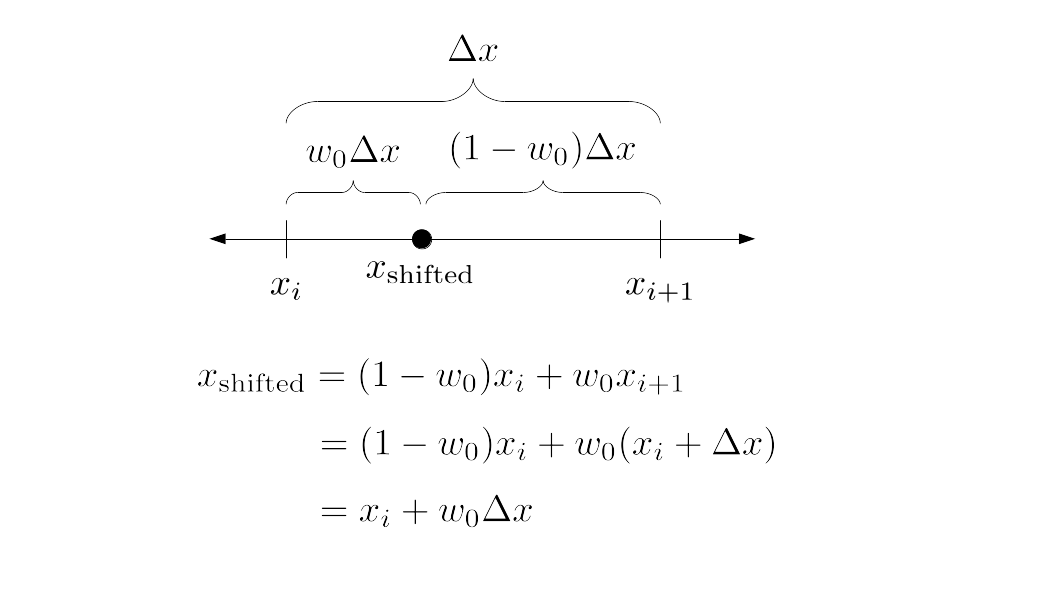
Now assume, like we did in the past, that there is a one-dimensional fluid flowing along this one-dimensional line. We would represent this fluid's velocity with a velocity vector at each grid cell boundary. So, suppose the fluid velocity at x_i is u_i and the fluid velocity at x_{i + 1} is u_{i + 1}. What is the fluid velocity at x_shifted?

Well, in real life, who knows? We'll assume in this tutorial that grid cells are small enough that no complicated variations in fluid flow happen within a single grid cell. (This is certainly not a universal assumption in fluid dynamics; for example, look up large-eddy simulation where you actually include a model of what happens at scales smaller than a grid cell!) So, let's just assume that within this grid cell, the fluid velocity varies linearly. In other words, just like the position of x_shifted is a linear combination of the positions of x_i and x_{i + 1}, let's assume the velocity of the fluid at x_shifted, which we shall denote by u_shifted, is also a linear combination of the fluid velocities at x_i and x_{i + 1}, which we shall denote by u_i and u_{i + 1}, respectively, with the same weights:

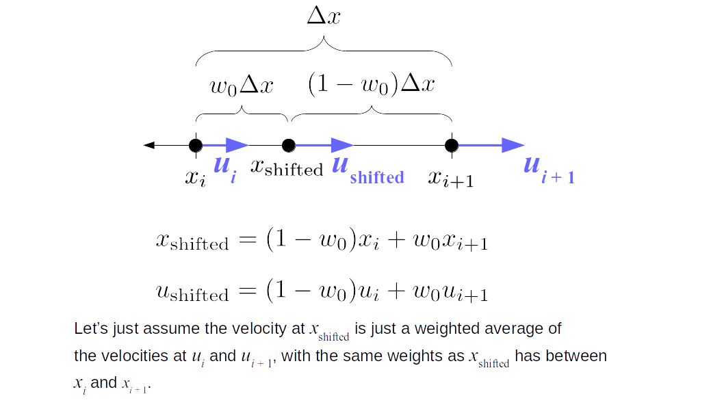
We explained the concept of advection earlier when introducing the Navier-Stokes momentum equation. So, how do we "advect" fluid velocity in 1D? We'll just draw imaginary grid cells around x_i, x_{i + 1}, and the particle's location, which we denote by x. A grid cell in 1D is just a closed interval of the real line of length Δx:

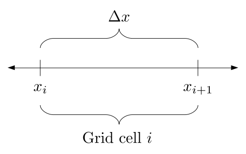
We'll assume the particle's velocity is just the fluid velocity at the particle's location, x, assuming velocity varies linearly between grid points. In other words, we'll look at what fraction of the particle-centered grid cell overlaps with the imaginary grid cell centered at x_i and what fraction of the particle-centered grid cell overlaps with the imaginary grid cell centered at x_{i + 1}:

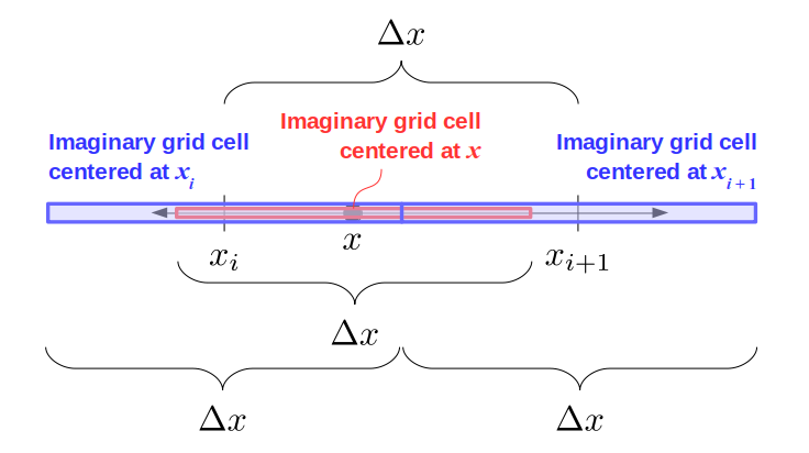
We'll assume the particle's velocity is just a weighted average of the velocities u_i and u_{i + 1} at the grid points around the particle, with the weights being these ratios of overlap. Once we have calculated the particle's velocity like that, we'll just multiply it by Δt and add it to the particle's current position, so that at time t + Δt, the particle will be located at x plus Δt times that velocity we just calculated. But okay that all sounds very fancy; exactly what are these weights, how do we figure them out, and what does the whole computation actually look like? Let's look at the same figure again but with the cells made thicker and with labels for the ends of the particle-centered cell and for the meeting point of the grid-point-centered cells:

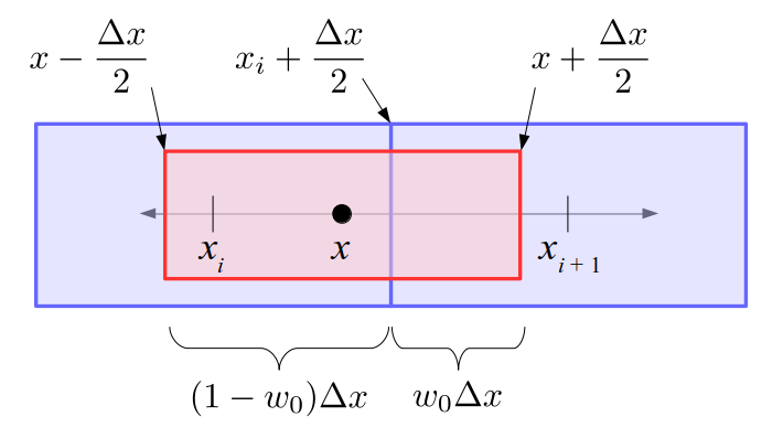
If we let w₀ be the ratio of distance of x from x_i versus distance of x_{i + 1} from x_i as in the earlier description of linear interpolation, then x - x_i = w₀Δx. That is, if w₀ = (x - x_i) / (x_{i + 1} - x_i), then noting that x_{i + 1} - x_i = Δx, then w₀ = (x - x_i) / Δx, so x - x_i = w₀Δx. See the earlier diagrams if you're confused about which points are separated by a distance of Δx, the width of a grid cell. Then the amount of overlap between the x-centered imaginary grid cell and the x_i-centered imaginary grid cell is (x_i + Δx/2) - (x - Δx/2) = x_i - x + Δx = -w₀Δx + Δx = (1 - w₀)Δx. Similarly, the length of overlap between the x-centered imaginary grid cell and the x_{i + 1}-centered imaginary grid cell is (x + Δx/2) - (x_i + Δx/2) = x - x_i = w₀Δx. This explains how the labels in the figure above are derived.

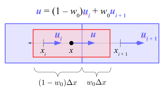
We assume the velocity of a particle located at x is the weighted average of the two grid velocities around it, with the weights being the fraction of overlap between the particle-centered imaginary grid cell and each velocity's imaginary grid cell. In this case, the fraction of the x_i-centered imaginary grid cell overlapped by the x-centered imaginary grid cell is 1 - w₀. So, we multiply 1 - w₀ by u_i and say that is the contribution of the fluid velocity, u_i, at grid point x_i, to the estimated velocity of the particle. The fraction of the x_{i + 1}-centered imaginary grid cell overlapped by the x-centered imaginary grid cell is w₀. So, we multiply w₀ by u_{i + 1} and say that is the contribution of the fluid velocity, u_{i + 1}, at grid point x_{i + 1}, to the estimated velocity of the particle. So, the total estimated velocity of the particle is u = (1 - w₀)u_i + w₀u_{i + 1}. In many ways this is the same logic as splatting, but in the opposite direction: going from grid velocities to a particle velocity based on the amount of overlap between a particle-centered cell and grid point-centered cells where velocities are located.

Once we have determined this velocity, u, for the particle, then advection would simply be updating the particle's position from x at time t to x + uΔt at time t + Δt. We used linear interpolation to calculate the particle's estimated velocity, u from the fluid velocity at neighboring grid points.

Note that the calculation of the grid cell overlap fractions above involves shifting half a grid cell width back from the particle's position to find the left end of the imaginary particle-centered grid cell, landing in either the particle's current cell or the cell to the left, just like we did with splatting. In this section I could have described the computation that way again, but I chose to just forget about which cell the left end of the particle-centered imaginary cell lies since the end result is still just the fraction of overlap between the particle-centered imaginary cell and the velocity-/grid-point-centered imaginary cells around it.

Advection in 2D

This works very similarly in 2D. We'll estimate the velocity of a particle first just for the horizontal grid velocities using bilinear interpolation, i.e., areas of overlap instead of lengths of overlap, and then once again for the vertical grid velocities.

Recall that when we did splatting in 2D we shifted downward by a half grid cell width to find the lowest y value of the imaginary particle-centered grid cell. We do the same thing here, but as with the 1D case above, I'll ignore which grid cell we end up in after that shift and just jump to the end result, which again is just the fraction of the imaginary particle-centered grid cell's overlap with its nearby grid-point-/velocity-centered grid cells.

For horizontal grid velocities, this is:

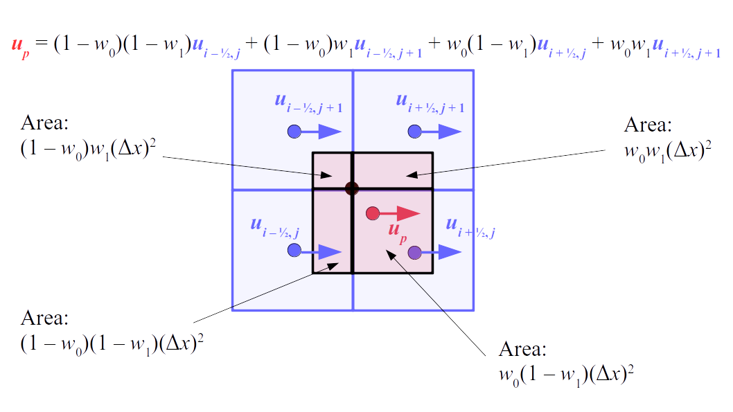
Changing the indices to integers as they would be in the code:

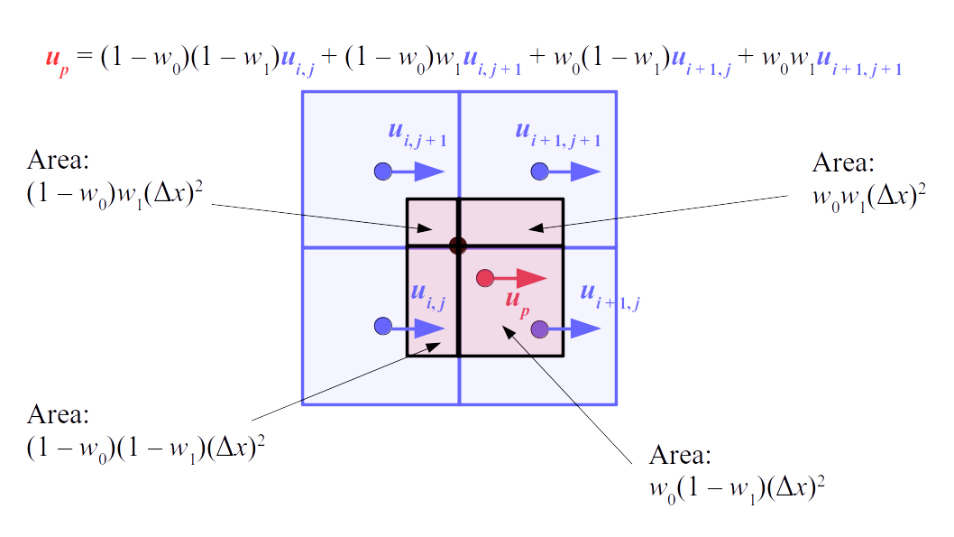
u_p in these figures is the horizontal component of the velocity we estimate for the particle based on the horizontal grid velocities. This calculation of overlap areas between these imaginary grid cells is identical to the calculation we did for splatting velocities in 2D. This computation where we essentially do linear interpolation in 2D instead of 1D to get the overlap areas is called bilinear interpolation.

Let's go a bit more step-by-step for the vertical velocities since we never illustrated them during the splatting section earlier. First, we shift leftward (the negative x direction) from the particle's location by half a grid cell width and compute the barycentric weights of the resulting position:

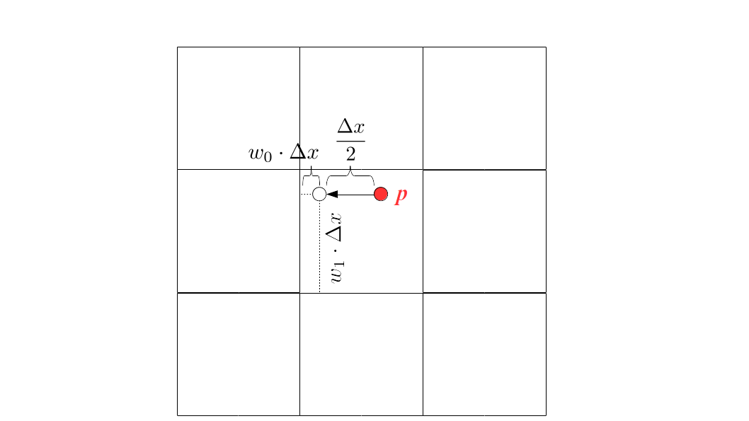
The vertical grid velocities are located at the horizontal boundaries between grid cells. The vertical grid velocities of interest are the ones around the particle's location:

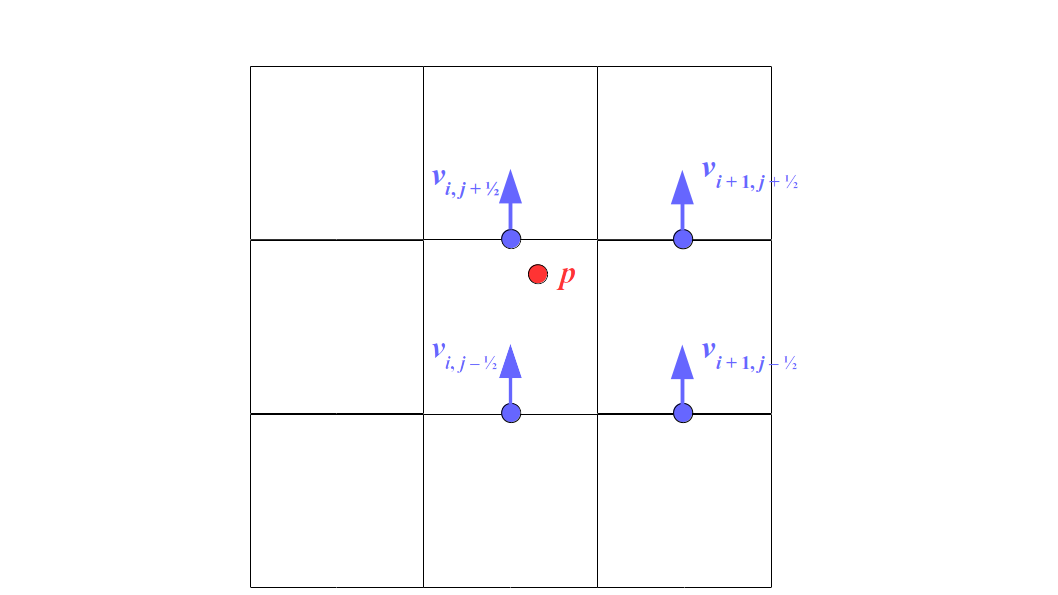
Now, let's draw imaginary grid cells around the points where each of those vertical velocities are defined:

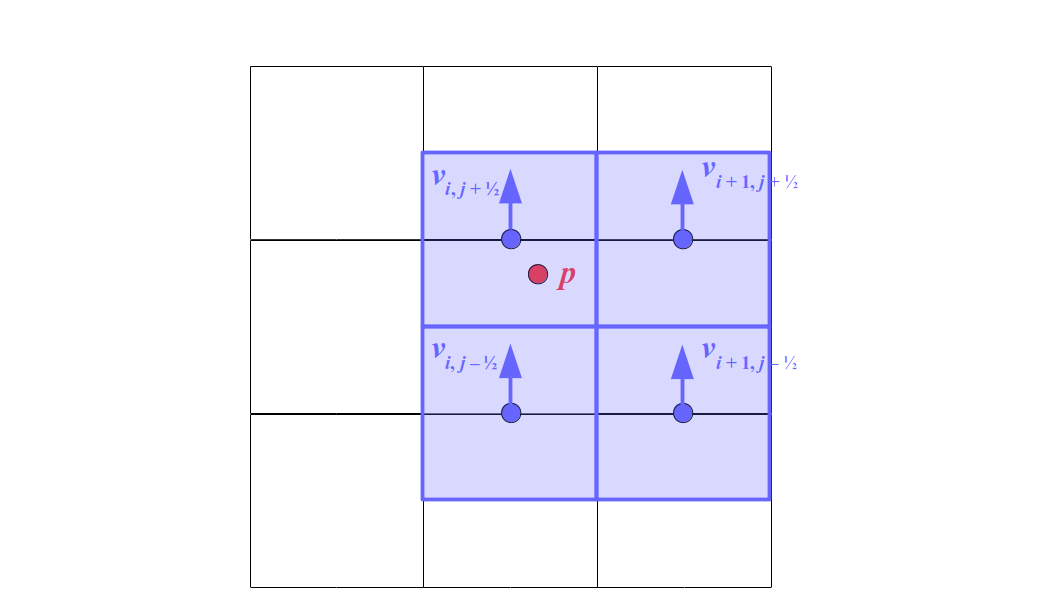
Then just like in the horizontal velocity case, the vertical component of the particle's velocity will be estimated, via bilinear interpolation of the barycentric weights of the shifted particle position, based on those vertical grid velocities:

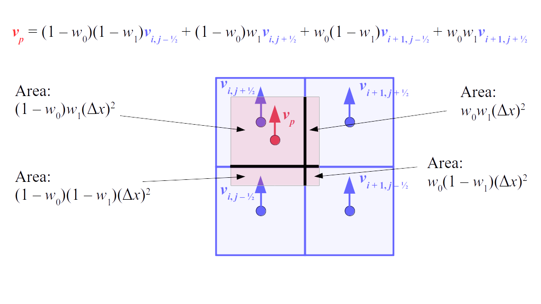
Or, removing the ½s and converting to the integer indices we'll use in our C++ code:

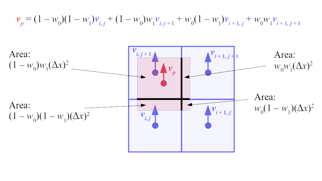
So, the resulting velocity of the particle that we'll use for advection is just (u_p, v_p). Our advection step is completed when we update the particle's position from its current position, x, to x + (u_p, v_p)Δt.

Notice something convenient above: the formula for u_p is exactly the same as the formula for v_p, but just with 'u's instead of 'v's! This is a consequence of our integer indexing scheme. We'll apply this same pattern in 3D in the next section.

Advection in 3D

I went through advection in 1D and 2D in great detail because I am absolutely not going to try to draw the 3D volumes of overlap for 3D advection. Instead, we'll just present the formulas and procedure without any illustrations. In 1D, we did linear interpolation using a barycentric weight to determine the particle's velocity for advection. In 2D, we used bilinear interpolation of a point's two barycentric weights. So, in 3D, we use trilinear interpolation using three barycentric weights to compute a velocity for each particle based on grid velocities.

The velocity we'll assign to a particle p, using the integer indices we'll use in our C++ code, will be (u_p, v_p, w_p) where u_p is

•    (1 - w₀) · (1 - w₁) · (1 - w₂) · u_{i, j, k}
• + (1 - w₀) · (1 - w₁) · w₂ · u_{i, j, k + 1}
• + (1 - w₀) · w₁ · (1 - w₂) · u_{i, j + 1, k}
• + (1 - w₀) · w₁ · w₂ · u_{i, j + 1, k + 1}
• + w₀ · (1 - w₁) · (1 - w₂) · u_{i + 1, j, k}
• + w₀ · (1 - w₁) · w₂ · u_{i + 1, j, k + 1}
• + w₀ · w₁ · (1 - w₂) · u_{i + 1, j + 1, k}
• + w₀ · w₁ · w₂ · u_{i + 1, j + 1, k + 1},

v_p is

•    (1 - w₀) · (1 - w₁) · (1 - w₂) · v_{i, j, k}
• + (1 - w₀) · (1 - w₁) · w₂ · v_{i, j, k + 1}
• + (1 - w₀) · w₁ · (1 - w₂) · v_{i, j + 1, k}
• + (1 - w₀) · w₁ · w₂ · v_{i, j + 1, k + 1}
• + w₀ · (1 - w₁) · (1 - w₂) · v_{i + 1, j, k}
• + w₀ · (1 - w₁) · w₂ · v_{i + 1, j, k + 1}
• + w₀ · w₁ · (1 - w₂) · v_{i + 1, j + 1, k}
• + w₀ · w₁ · w₂ · v_{i + 1, j + 1, k + 1},

and w_p is

•    (1 - w₀) · (1 - w₁) · (1 - w₂) · w_{i, j, k}
• + (1 - w₀) · (1 - w₁) · w₂ · w_{i, j, k + 1}
• + (1 - w₀) · w₁ · (1 - w₂) · w_{i, j + 1, k}
• + (1 - w₀) · w₁ · w₂ · w_{i, j + 1, k + 1}
• + w₀ · (1 - w₁) · (1 - w₂) · w_{i + 1, j, k}
• + w₀ · (1 - w₁) · w₂ · w_{i + 1, j, k + 1}
• + w₀ · w₁ · (1 - w₂) · w_{i + 1, j + 1, k}
• + w₀ · w₁ · w₂ · w_{i + 1, j + 1, k + 1}.

Notice how the indices and interpolation calculations are identical for u, v, and w. In other words, if we had a single function to calculate this trilinear interpolation of velocity values for a given grid cell index, (i, j, k), then we could simply pass the appropriate 3D array, u, v, or w, into that function to get the trilinearly interpolated velocity component we want. Once we have done this trilinear interpolation for u, v, and w for each particle's position, x ∈ R³, we then compute the particle's position at the next time step as x + (u_p, v_p, w_p)Δt.

Recall that we labeled grid cells on the boundary of the grid as SOLID. That means fluid particles should never move into the solid grid cells. So, let's also add a step to our advection algorithm here: if the computed particle position at the next time step, x + (u_p, v_p, w_p)Δt, goes beyond the outermost non-SOLID grid cells, then let's set the particle to the farthest out coordinate values it can possibly have, with a tiny extra buffer room to deal with the precision errors that can occur with floating-point numbers.

Implementing 3D Advection

Copy the code from the incremental2 folder to a new incremental3 folder. Based on the algorithm description above, we add an Advect function to the StaggeredGrid class that takes a single Particle's position and returns the position at the next time step that results from advection of the fluid velocity at that particle's location, which itself is computed via trilinear interpolation as above. The new Advect function is added to StaggeredGrid.h and StaggeredGrid.cpp. A test of the advection code is added to StaggeredGridTest.cpp. Note that our test does not check whether the code correctly clamped the particle positions to the non-solid cells after advection. I simply neglected to add this earlier and decided to leave it untested for now.

Compile and run this code just like you did for the code in the incremental2 folder earlier. Clean it up by deleting a.out when you're done running it.

Applying Body Forces

The forces resulting from internal pressure and viscosity of a fluid are two of the terms in the Navier-Stokes momentum equation governing our fluid flow model. Another term is the body forces term, which is often just a gravity term. In our fluid simulation, we'll simply apply a gravitational acceleration throughout our fluid by subtracting Δt · 9.80665 m/s² from all vertical velocities in our staggered grid. Accordingly, we make a copy of our directory, incremental3, called incremental4, in which we update StaggeredGrid.h, StaggeredGrid.cpp, and StaggeredGridTest.cpp to include and test a new function, ApplyGravity, which applies exactly this subtraction to the grid's vertical velocities.

Compile and run this code just like you did for the code in the incremental2 and incremental3 folders earlier. Clean it up by deleting a.out when you're done running it.

Note that our changes to the grid velocities will likely not meet our boundary conditions we described earlier during splatting. So, we call the same function to fix the boundary velocities that we did during splatting, after applying gravitational acceleration to our vertical velocities!

Pressure Projection

So far we have added the effects of the advection term and the body forces (gravity) term. We will now incorporate the pressure term and the incompressibility constraint. Recall that the pressure projection step is intended to compute a pressure function for our fluid that causes its velocity field to be divergence-free, or volume-conserving. Conceptually, the purpose of pressure is to conserve volume, and recalling that the incompressibility a.k.a. zero-divergence a.k.a. volume-conserving constraint was just a simplication of mass conservation, we can say the purpose of pressure is to conserve the mass of the fluid.

Velocity Update via the Discrete Pressure Gradient

As explained in Chapter 4 of Bridson and Müller-Fischer's course notes, we split our Euler equations so that we started with an initial velocity field, then found a velocity field that incorporates the advection term, and then found a velocity field that incorporates the gravity term. Now, we want to solve the equation ∂u/∂t = -(1/ρ)∇p by discretizing it to (u_next - u) / Δt = -(1/ρ)(p_next - p) / Δx, and find a pressure field p such that solving for the next time step's velocity field u_next satisfies the incompressibility constraint ∇ · u_next = 0 and the solid wall boundary conditions. The idea here is that the "current" velocity field u already incorporated the advection and gravity terms from the Euler momentum equation, so we pretend the only term we have left to add is the pressure gradient term subject to the incompressibility constraint. Notice in that discretized version of the remaining terms in the Euler momentum equation, u_next refers to the next velocity temporally, i.e., at the next time step while p_next refers to the next pressure spatially, e.g., in an adjacent grid cell. That is, u really means u(x, y, z, t) and u_next is really shorthand for u(x, y, z, t + Δt), p is p(x, y, z, t), and p_next is shorthand for p(x + Δx, y + Δx, z + Δx, t). Solving for u_next in the discretized differential equation yields u_next = u - (Δt/ρ)(p_next - p) / Δx. But in the staggered grid we break this all up by dimension. First, let's examine a cell (i, j, k) and its neighbors to the right, top, and front and recall that the pressure value for each grid cell represents the fluid pressure at the cell's center:

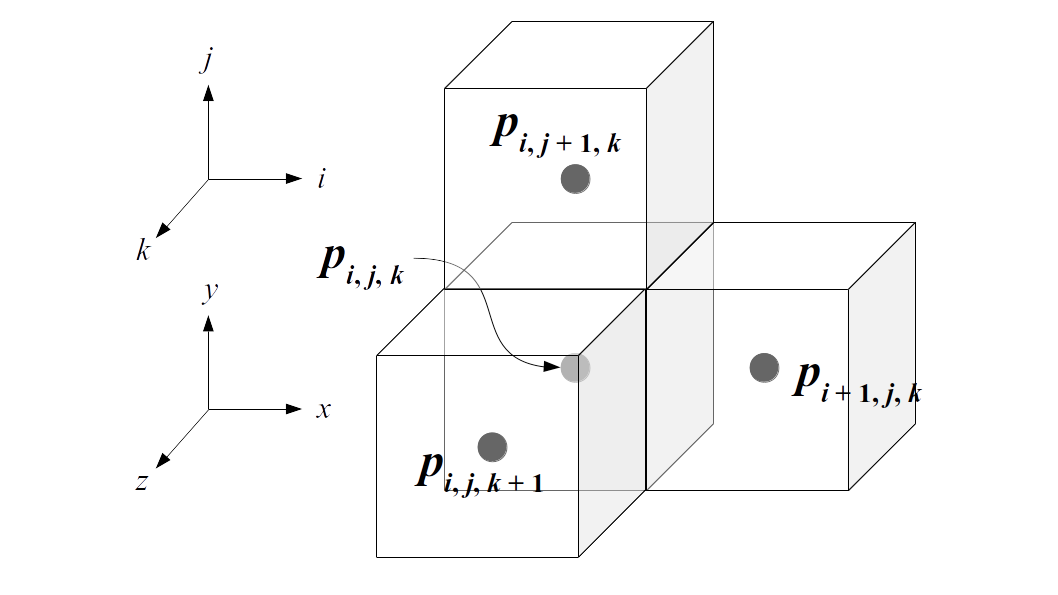
Then, assuming we have already found a pressure function that makes the velocity field divergence-free, the fluid velocities at the next time step in the grid, for any fluid velocity bordering a grid cell marked as containing fluid, are:

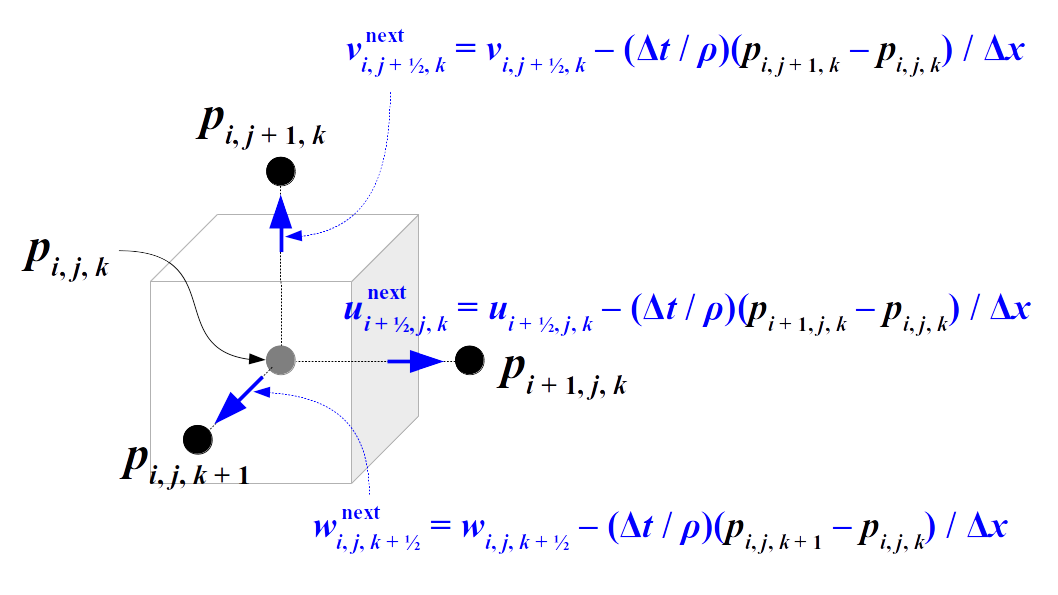
Discrete Divergence of the Velocity Field

The velocity field's divergence is ∇ · u = ∂u/∂x + ∂u/∂y + ∂u/∂z. Discretizing the three spatial derivatives on the right-hand side of that equation, across any grid cell marked as a fluid gives us the discrete divergence of the velocity field for cell (i, j, k) shown in the figure below. This is where the staggered grid becomes very useful. Notice how the discrete divergence of the fluid velocity is just computed by subtracting stored grid velocities, dividing by the grid cell width, and adding these values together for each dimension!

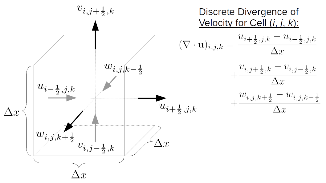
Since the incompressibility constraint states that the divergence of the velocity field should be zero, we can substitute the pressure-based velocity update equations in the previous section into the next time step's velocity variables (the variables labeled with "next"):

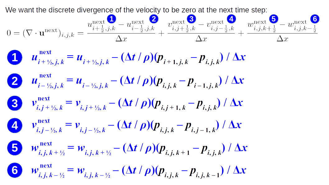
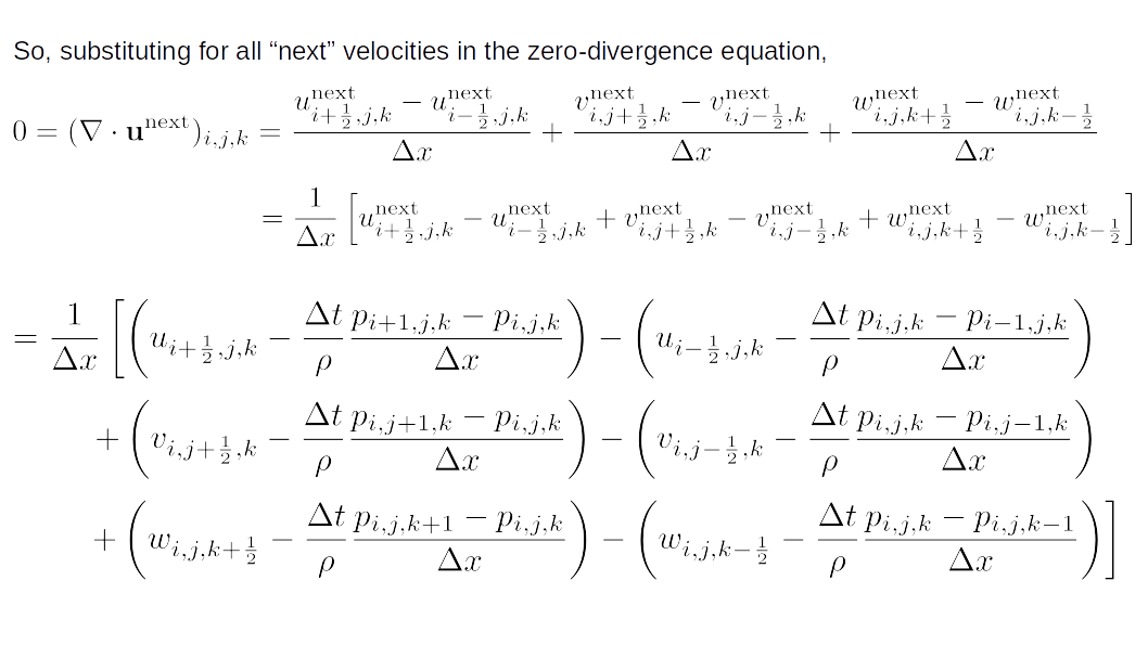
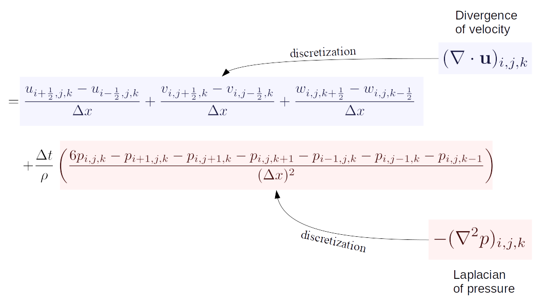
This derivation is explained in Bridson and Müller-Fischer's course notes in Section 4.3. The observation that the last term above contains a discretization of the Laplacian of pressure is justified following the standard seven-point stencil central difference approximation of the Laplacian as a derivative of derivatives. The central differencing scheme for second derivatives is described for one and two dimensions in Bargteil and Shinar's course notes on pages 31-32. Here is how we can derive the seven-point stencil-based central difference approximation of the Laplacian of our fluid's pressure:

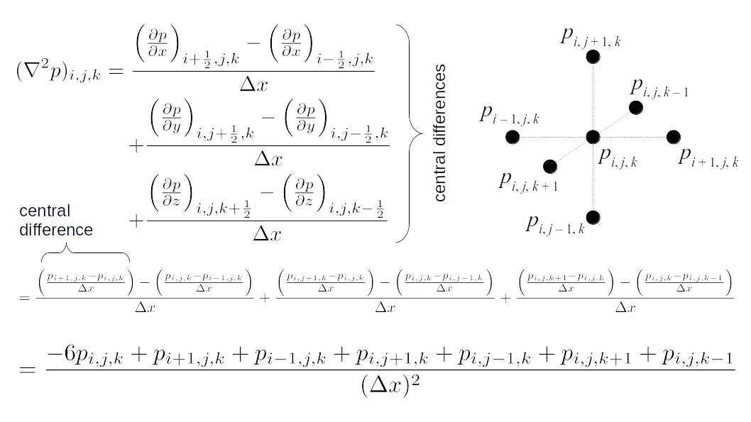
Let's move velocity terms to one side of the pressure-based zero-divergence equation we derived above. That leaves us with:

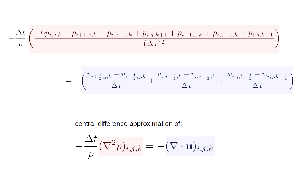
We can divide through by Δt/(ρ(Δx)²) and distribute the negative sign through the pressure terms to get:

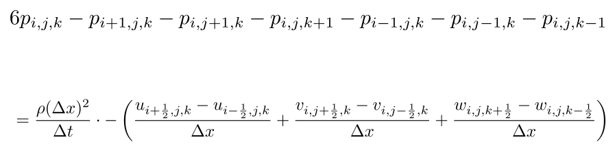
Since this equation applies to all cells (i, j, k) labeled as fluid, this actually is a whole system of linear equations with all the pressure values being the unknown values stacked into a single vector, p, and all other values being known. The scaled divergences on the right-hand side can be stacked into a single vector, d:

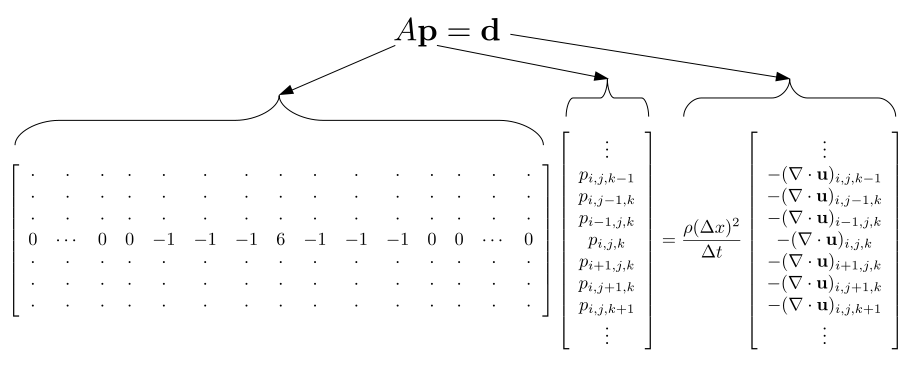
We can write this as a linear equation Ap = d, where A is a matrix containing six -1s and one 6 in each row corresponding to a fluid grid cell. This is a large, sparse matrix since other than those -1s and 6s in each row corresponding to a fluid cell, the entire matrix is full of zeros.

As described in Bridson and Müller-Fischer's course notes, in case of an empty neighboring cell, we simply set that neighbor's entry in matrix A to zero instead of -1. In case of neighboring cells being solid, we reduce the 6 by however many solid neighboring cells are present. So, in general, the "6" is actually just the number of non-solid grid cell neighbors of cell (i, j, k).

Conjugate Gradient Algorithm

Our goal is to solve the equation above, Ap = d, for p. We already know d: those are just the scaled negated divergences from the current (old) time. The matrix A is also known, big, and sparse. Wouldn't it be nice if we could just invert A and get p = A^-1d in one step, and be done? Unfortunately, A is not always invertible, and being large and sparse, storing the matrix and directly inverting it requires storing a lot of unnecessary information. Fortunately, A is also symmetric and positive-semi-definite, so there's another easy-to-implement algorithm we can use to solve this problem: the Conjugate Gradient Algorithm, without even requiring us to store the actual A matrix anywhere in computer memory during our program's execution!

This very approachable, yet detailed introduction to the Conjugate Gradient Algorithm by Dr. Jonathan Shewchuk lists the steps of the algorithm on page 32, while the rest of the document explains the algorithm, variations on it, its derivation, and its properties. Here we will describe and illustrate a summary of what is described in Dr. Shewchuk's document. Page 34 of Bridson and Müller-Fischer's course notes also lists a similar algorithm called the Preconditioned Conjugate Gradient Algorithm, which is not what we're using in this tutorial (we're just doing the regular, vanilla Conjugate Gradient Algorithm), but shows the criteria for when to stop the algorithm from repeating iterations of its calculations.

The Conjugate Gradient Algorithm takes advantage of the fact that you can write a function called a quadratic form using A, p, and d, whose graph is a giant bowl if A is positive-definite, where c is some real number:

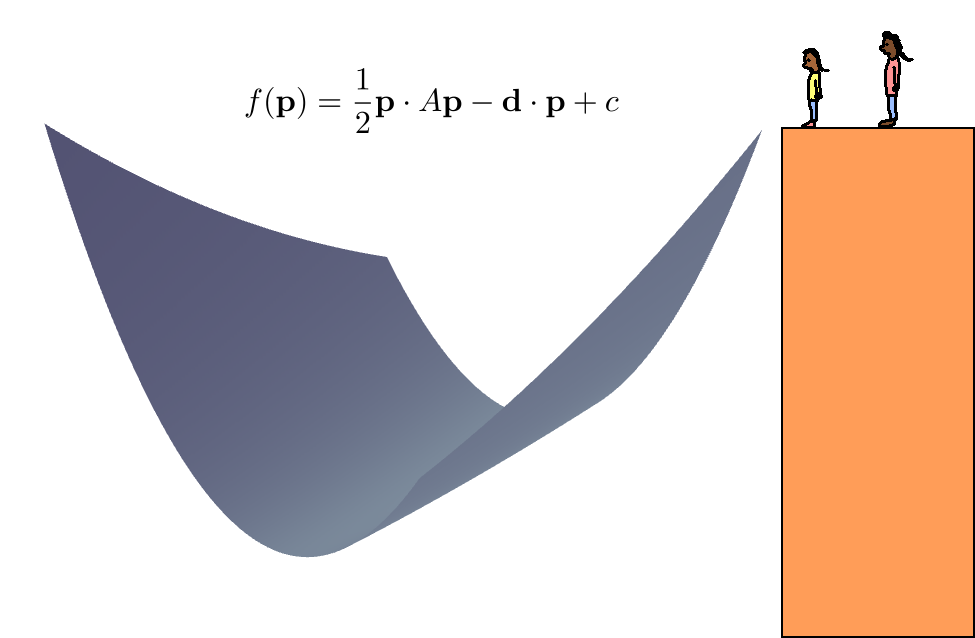
(If A is positive semi-definite, we can still use the same algorithm.) The idea is to pick some initial guess at a solution, p₀:

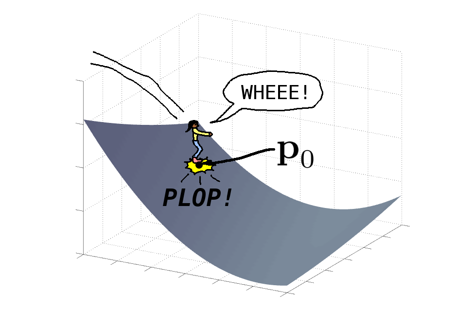
As Bridson and Müller-Fischer describe, we can just start with a guess of all zeros, p₀ = 0 since, for example, some more "intelligent" approach like using a previous time steps' pressures may not work since some grid cells may have switched to or from even being fluid. Then, figure out how far you are from the bottom of the bowl. Well, we don't know what p vector will actually get us to the bottom of the bowl, but we do know that whatever that correct p is, left-multiplying it by A gives us d since that was the equation we started with: Ap = d! So, how far we are from the correct solution to Ap = d can be measured using the residual vector, r₀ = d - Ap₀, based on our initial guess, p₀:

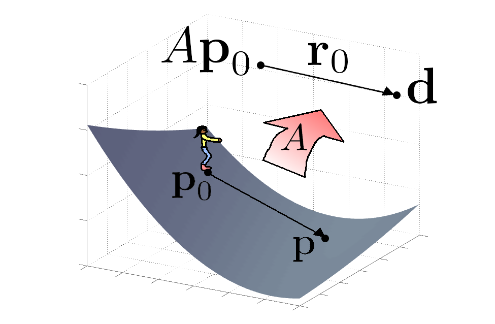
Well, now that we know how far we are from the correct solution, let's figure out how to get closer to the solution! We're going to take a step toward that solution. But how big a step, and in what direction? It turns out, the step direction, d₀, can just be the residual, r₀, which takes us in a direction closing the gap between our current guess, p₀, and the final solution, p. The step size is calculated in terms of the matrix, residual, and step direction as α₀ = r₀ · r₀ / (d₀ · Ad₀). That takes us to a new guess at the solution, p₁ = p₀ + α₀d₀:

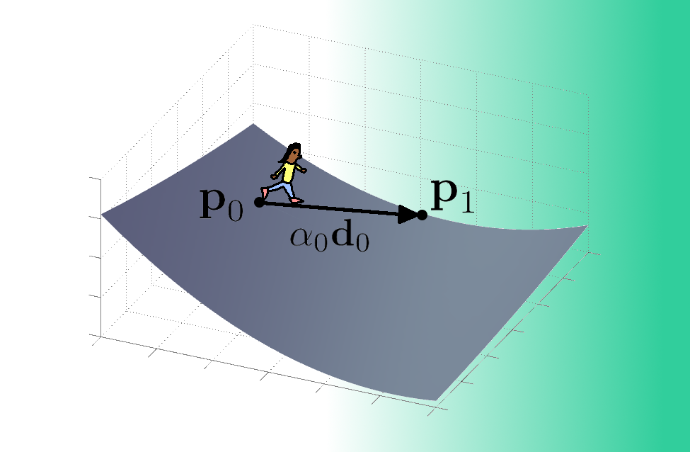
The new residual, or how "off" we are from the solution's scaled, flipped divergence values, is updated to r₁ = r₀ - α₀Ad₀:

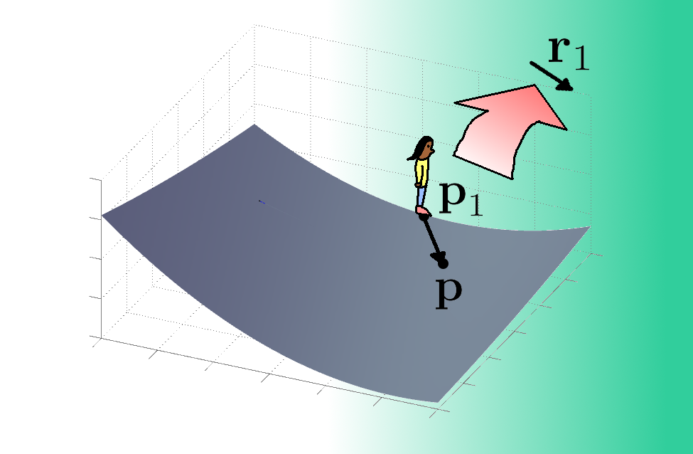
We then compute how small our new residual's magnitude is relative to the previous residual, β₁ = (r₁ · r₁) / (r₀ · r₀). From this, we determine the next direction in which to step: d₁ = r₁ + β₁d₀:

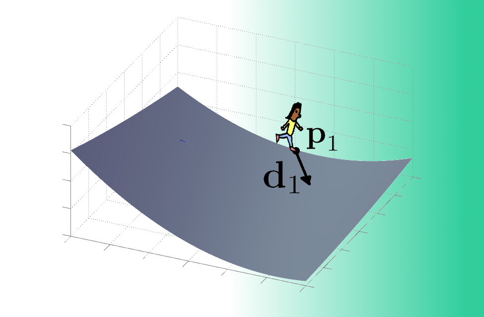
This process repeats with computing the next step size, α₁, the new solution guess, p₂, etc.

But when does this process end? How many steps should we end up taking? Well, as Bridson and Müller-Fischer describe, we can arbitrarily stop when we either get close enough to the solution (we'll say if the sum of squared scaled, flipped divergences of our current solution guess is no more than 10^-6 times the sum of squared original scaled, flipped divergences) to declare that we're done, or when we're taken a certain number of steps toward the solution (we'll say a thousand), we're done. This entire process of taking up to a thousand steps to end within one time step of our simulation, so we don't want it taking forever!

Thus, we end up with the algorithm described in Shewchuk's document, which is also how the algorithm is implemented in Bargteil and Shinar's code (note all equals signs are assignment statements, not statements of truth!):

• Start with p = 0.
• Start with r = d, i.e., the starting residual should equal the starting step direction.
• Compute the squared magnitude of the residual: σ = r · r.
• Set the threshold for how close we want to get to the ideal solution, tolerance = 10^-6 · σ.
• Repeat until 1000 steps are taken or σ ≤ tolerance:
  • Set the matrix-mapped step direction to be q = Ad.
  • Set the step size, α = σ / d · q.
  • Move to the new solution guess, p += αd.
  • Compute the new residual, r -= αq.
  • Save a copy of the old residual's magnitude, σ_old = σ.
  • Compute the squared magnitude of the new residual, σ = r · r.
  • Compute how small the new residual is relative to the old one, β = σ / σ_old.
  • Set the new step direction based on the old step direction: d = r + βd.

Implementing Pressure Projection

Now we have all the steps in place for handling the pressure gradient term of the Euler momentum equation: compute the scaled, flipped divergences of our fluid's grid velocities, use the Conjugate Gradient Algorithm to compute pressure values that minimize the divergence of an updated grid velocities, and then subtract the resulting pressure gradient (for all non-SOLID grid cells) to obtain the new grid velocities.

Before we apply the Conjugate Gradient Algorithm though, we need a way to compute the effect of multiplying pressures by the matrix A without actually storing that matrix: it's sparse and huge, so we can compute it more efficiently if we just compute and store information on neighbors of fluid grid cells so we know what numbers to use for each row of the matrix.

Exactly what do we need to know about grid cells' neighbors? First, since we're only interested in fluid grid cells, we can skip all the cells on the outer boundary of our grid on all sides, since those are all cells marked as SOLID. So, we can restrict ourselves to the grid cells with indices (i, j, k) where 1 ≤ i ≤ n_x - 1, 1 ≤ j ≤ n_y - 1, and 1 ≤ k ≤ n_z - 1. We can also skip any grid cell that is not labeled as FLUID. For each remaining cell, look at its six neighbors above, below, left, right, behind, and in front of the cell. First, count how many of those six neighbors are either marked as FLUID or EMPTY themselves. Second, we want to remember which of these six neighbors is actually FLUID, and not EMPTY. Why do we need this information? Because we will use it to "multiply a vector by the matrix A" without actually storing A itself or doing any actual matrix multiplication: for each cell (i, j, k), if the cell has no fluid or empty neighbors, we'll skip it entirely; otherwise, we'll multiply the (not-stored-anywhere) matrix A times a vector d by first multiplying by the entry for cell (i, j, k) in the vector d by the number of the cell's non-SOLID neighbors (this corresponds to the number 6 we showed in the A matrix example earlier for any cell that has all 6 neighbor cells being non-SOLID) and then subtracting the entry for each FLUID neighbor cell in the vector d (this corresponds to each -1 entry in a row of the matrix A).

Okay, but how shall we store all this data? Keeping count of the neighbors of each cell as well as keeping track of up to 6 neighbors of each cell in the entire grid seems like a lot of data to store! Well, we can use bit manipulation to minimize storage. Since we can have up to six non-SOLID neighbors of any given grid cell, well, the number 6 is 110 in binary, so we need three bits to store the number of non-SOLID neighbors of a grid cell. Then, for each of those six neighbors, we want to store a single bit that is 1 if that neighbor cell is FLUID, and 0 otherwise. So that's one bit for each of the six neighbors, so six more bits we need to store. So, we need to store a total of three bits for the number of non-SOLID neighbors of a cell and six bits for the number of FLUID neighbors, so that's 3 + 6 = 9 bits total that we need to store. Now, we could store all of this information for all grid cells in our entire grid by creating a 3D array of a 9-bit std::bitset object, but to keep things simple and avoid possible overhead from using another data structure just for this, let's just store this as a 3D array of integers that can store at least 9 bits. There is no built-in 9-bit integer data type in C++, so we use the smallest built-in integer type that contains 9 bits, which is the 16-bit unsigned integer type, unsigned short:

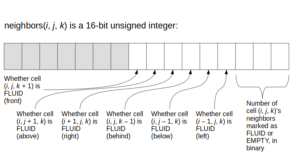
Here is a diagram of where those neighbor cells are relative to the cell (i, j, k), which is the unlabeled cell in the middle:

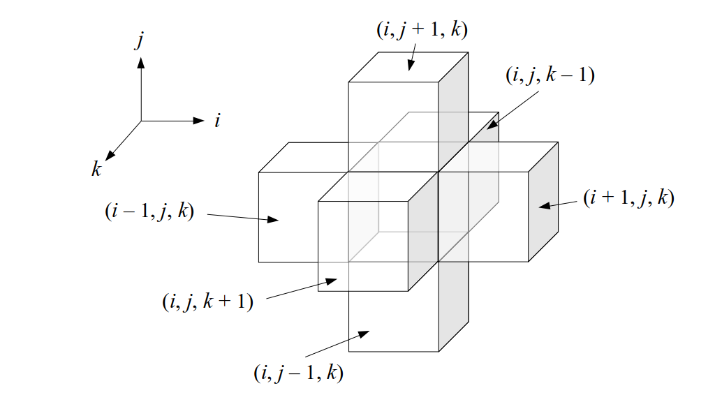
As an example, if the fluid cell at index (3, 5, 2) has six fluid cell neighbors, the entry in this 3D array neighbors at index (3, 5, 2) will look like this:

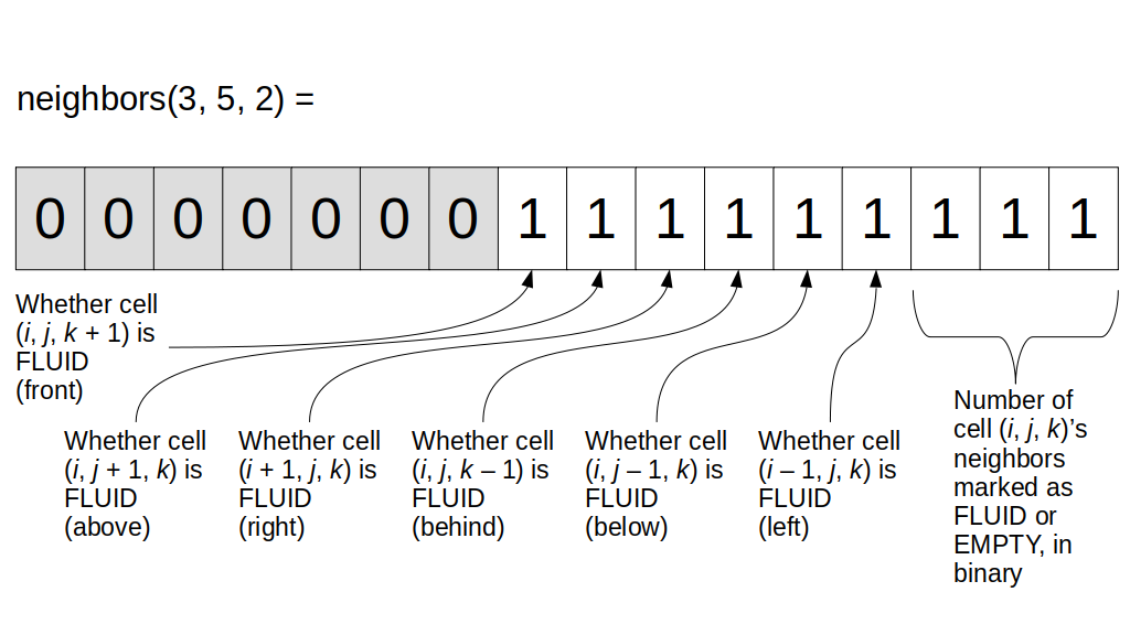
On the other hand, if the fluid cell at index (5, 0, 18) has three fluid neighbors on its right, above it, and to its left, two empty neighbors below it and in front of it, and a solid neighbor behind it, the entry in this 3D array neighbors at index (5, 0, 18) will look like this:

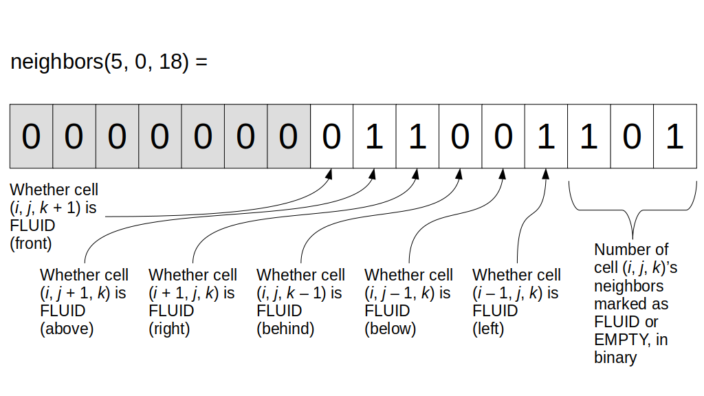
And that's it! So, just storing and updating these 9 bits of information for each grid cell in each time step allows us to multiply the giant, sparse matrix A by any vector without ever storing the array anywhere or doing any fancy matrix multiplications! We just iterate through all the grid cells, count neighbors, and multiply and subtract some stuff, and we're done!

Here is our implementation of pressure projection! The entire implementation is in the incremental5 directory. We updated Array3D.h to include functions SetEqualTo, PlusEquals, EqualsPlusTimes, and Dot to allow doing arithmetic using whole 3D arrays. In the StaggeredGrid class, we added the ProjectPressure function that generates the neighbors array we described above based on the material type of each grid cell, applies the Conjugate Gradient Algorithm to compute pressure values that lead to a sufficiently divergence-free fluid velocity in the grid, and then updates the velocity based on the resulting pressure gradient, just as we described above. A separate class, PressureSolver, is introduced to implement the Conjugate Gradient Algorithm to solve for pressure. The logic behind the introduction of this class is that the main StaggeredGrid class will never need access to the objects used for the Conjugate Gradient Algorithm such as the residual vector (stored as a 3D array in the code since the "vector" would contain exactly one value per grid cell, and our per-grid-cell values in general are already stored using 3D arrays), so it makes sense to encapsulate those objects into the PressureSolver class, which is the only class that will ever access or modify those objects. Note we do not use return value optimization in the PressureSolver code even though we have functions whose sole job is to return a 3D array of values, since we will not be creating and destroying the 3D arrays that receive the 3D arrays that would be "created" and returned by those functions--they are relatively large objects so we choose to keep them in memory throughout the fluid simulation and simply update their values in each time step (e.g., the 3D arrays for residuals and pressures) rather than creating and destroying them on the stack repeatedly.

To compile the code in the incremental5 directory, cd to that directory in a terminal window and execute this command:

g++ jsoncpp.cpp Particle.cpp PressureSolver.cpp SimulationParameters.cpp StaggeredGrid.cpp StaggeredGridTest.cpp -I/usr/include/eigen3/

Run the StaggeredGridTest.cpp code with the same command as earlier:

./a.out inputs/fluid.json

Then clean up as usual:

rm a.out

Mapping from the Grid to the Particles

The last major computation in a time step of our simulation is the transfer of fluid velocities from the grid back onto the fluid particles. The Particle-in-Cell (PIC) algorithm interpolates the velocities on the grid closest to the position of a particle and assigns that interpolated value to be the particle's new velocity. Since PIC interpolates velocities to transfer velocities from particles to the grid at the beginning of a time step (as we did earlier), and interpolates velocities again to transfer velocities from the grid back to the particles, this repeated interpolation of velocities tends to average or smooth out the velocities. In fluid simulation, the words "averaging," "smoothing," "dissipating," "damping," and "viscosity" all refer to the same phenomenon: the tendency to drive fluid velocities down to zero. This means PIC tends to suppress splashing or turbulent motion to a large extent, leading to potentially unrealistic simulations especially for fluids we assume have zero viscosity, as we did here, and as we often do in computer graphics.

The Fluid-Implicit-Particle (FLIP) method does the same thing, but with a slight modification for the grid-to-particle mapping: instead of updating particle velocities by setting them equal to interpolated grid velocities, it updates particle velocities based on change in interpolated grid velocities. As a result, FLIP doesn't have the same filtering or smoothing tendency of PIC, so it can preserve more of the inviscid, splashing, turbulent behavior of fluids. However, the downside of this is, FLIP can tend to be more unstable.

As a result, it's common to blend PIC and FLIP grid-to-particle updates to get the more accurate, dynamic fluid behavior of FLIP, while including a little bit of PIC's tendency to smooth out noise so things don't get too unstable. The resulting blended algorithm is what we call PIC/FLIP. To update the velocity of a particle, we save the grid velocities from before we applied boundary conditions, gravitational acceleration, and pressure projection, interpolate the grid velocities for the particle's location, and then do the same interpolation with the grid velocities from after applying boundary conditions, gravitational acceleration, and pressure projection. We then add the change in interpolated grid velocities to the particle's existing velocity. But to blend the PIC and FLIP strategies, we include a constant called the FLIP ratio. If u_p is the current velocity of a particle p, u_old is the interpolated grid velocity at the particle's position using the "before" velocities, and u_new is the interpolated grid velocity at the particle's position using the "after" velocities, and f is the FLIP ratio, then the new velocity of the particle is set to u_p = f(u_p - u_old) + u_new. We constrain the FLIP ratio so that 0 ≤ f ≤ 1. If f = 0, then we're doing a pure PIC algorithm: u_p = 0 · (u_p - u_old) + u_new = u_new, i.e., we're just setting the particle's new velocity equal to the newly interpolated grid velocities, with no consideration for how the grid velocities have changed during this time step. On the other hand, if f = 1, we're doing a pure FLIP algorithm: u_p = 1 · (u_p - u_old) + u_new = u_p + (u_new - u_old), where this subtraction in parentheses is the change in interpolated grid velocities we mentioned earlier. If 0 < f < 1, then we're doing a hybrid PIC/FLIP algorithm. In this tutorial, we happen to set f = 1 in our example input simulation parameters, so we are running a pure FLIP simulation; however, you can change the FLIP ratio in the inputs/fluid.json file to change this to a pure PIC simulation or a hybrid PIC/FLIP simulation.

The code for implementing and testing the PIC/FLIP grid-to-particle velocity transfer is demonstrated in a new directory, incremental6. The only files we've changed relative to the incremental5 directory are the StaggeredGrid.h, StaggeredGrid.cpp, and StaggeredGridTest.cpp files. Since we had some grid velocity interpolation code earlier for particle velocity advection, we've created a general function, InterpolateTheseGridVelocities, that can take any three 3D arrays of grid velocity components and interpolate the velocities for any given position in space. We then repurpose the fu_, fv_, and fw_ 3D arrays that we used earlier within the ParticlesToGrid function to store the barycentric weight sums to now store the actual grid velocities we get immediately after splatting and normalizing the grid velocities and before we apply boundary conditions or gravity or pressure projection. Then we simply call InterpolateTheseGridVelocities with fu_, fv_, and fw_ to get the "old" interpolated grid velocities. We call InterpolateTheseGridVelocities with u_, v_, and w_ to get the "new" interpolated grid velocities. In StaggeredGridTest.cpp, we demonstrate how we call our new GridToParticle function in the StaggeredGrid class to calculate a new velocity for each fluid particle. We test that we get the correct particle velocities when doing a pure PIC simulation, a pure FLIP simulation, and a hybrid PIC/FLIP simulation. A paper that nicely describes the theory behind PIC and FLIP updates is Hammerquist and Nairn (2017).

Finish the Simulation

Our goal now is to synthesize all the information above to create a complete fluid simulation program and perform a basic visualization of the fluid particle positions over time.

Fluid Simulation Driver

All this time we've been adding steps to the StaggeredGrid class and then testing them in StaggeredGridTest.cpp. But how do we go from testing our code to actually implementing and running a complete fluid simulation? And how do we actually see what the simulation looks like?

It turns out we can make a copy of our StaggeredGridTest.cpp code and make very small changes to it to make it run a complete fluid simulation. Then, with a bit of extra code we can save the resulting particle positions at each time step to output files. And then, using the strategy of visualizing particles as spheres in OpenGL as we did at the beginning of this tutorial, we can display all of the particles at all of these positions throughout the fluid simulation to visualize our fluid particles splashing around over time!

In a new directory, incremental7, we copy the code from incremental6 and create a new program, FluidSimulator.cpp, derived from StaggeredGridTest.cpp and following the structure of the main() function implemented in Bargteil and Shinar's fluid.cpp file. This file acts as the driver program for our complete fluid simulation.

Visualizing the Fluid Animation

One useful design decision, as demonstrated by Dr. Bargteil and Dr. Shinar's FLIP code, is to separate the fluid particle position computation code from the visualization code, so that our simulation calculations are not slowed down by the need to visualize arbitrarily large numbers of spheres.

We have slightly modified the particle viewer program provided with Bargteil and Shinar's code to make the particles look more blue and to save a snapshot image of each frame of our simulation as a .png file. These images can then be used to generate a movie or animated GIF of the simulation, as shown in the HOW_TO_RUN file provided with the code.

Also added to the incremental7 directory is a Makefile, which relieves us of having to remember all the g++ commands for compiling our programs. To run the scripts to generate a .mp4 movie file or an animated GIF of the simulation, you'll need to have the freely available FFmpeg program installed; search online for instructions on how to do it for your computer's operating system. On Ubuntu, I believe sudo apt install ffmpeg suffices in most cases.

The End Result

Video made using the FLIP solver we implemented in this tutorial!

Here is the simulation that results from running our code via the steps in the HOW_TO_RUN file! This image was actually generated using the GenerateGIF script provided with the code in that directory.

Now, if you've run Bargteil and Shinar's code before, you may notice a slight difference in their simulation vs. the one we created here:

Video made using the FLIP solver and visualizer in the SIGGRAPH physics-based animation course on which this tutorial is based.

Specifically, a fluid particle hovers above the main fluid surface a bit longer in our simulation than in theirs. Why? It turns out we used 9.80665 m/s² for our acceleration due to gravity value, while they use 9.8. Changing ours to 9.8 makes our simulation appear more visually identical to theirs.

Debugging a Fluid Simulation

Well, I may have given you the impression that with all the test code we wrote, we ensured that we have no bugs in our code. This is a lie! In fact, there were a few issues our tests did not catch the first time I implemented the code for this tutorial. I had to go back and fix the bugs I found in all of the relevant incremental* directories above. So, what were the bugs, how did I catch and fix them, and how might we prevent or deal with bugs in fluid simulators in general?

The first time I ran this complete fluid simulation, it crashed pretty quickly! Now the issue with fluid simulations is that there are a lot of quantities interacting and influencing each other, so simply using a traditional debugger and stepping through code one line at a time manually is going to be extremely tedious and ineffective, especially if your program crashes after numerous repetitions of parts of the code. Instead, the strategy I used is generate as much data as possible! The more data you have, the more information you have from which to determine what goes wrong and when.

The first bug I found was in my pressure solver code. The line originally read double sigma = Dot(r_, r_);, which accidentally created a new local variable inside the loop that would disappear at the end of each iteration of the loop! We actually wanted to just reuse the same sigma variable declared before the loop, so we could keep updating it and seeing if it gets small enough to land within the tolerance value. I had to fix this here and in the incremental6 directory.

But then I discovered another bug in the Normalize*Velocities functions in the StaggeredGrid class. Namely, I forgot to include the first nested loop in each of those functions that sets the boundary velocities to zero. I had to fix this bug in all directories going back to incremental2! Once I fixed this and the sigma declaration bug above, my simulation finally ran to completion. I tracked down this bug by printing out lots of data: grid velocities, particle positions and velocities, pressures, cell material types, cell neighbor information, residual values, etc., in every time step for some range of times, from both my code and Bargteil and Shinar's code to identify at what point the values in each program begin to differ from each other. I saved most of this data to different files and used the diff command in many cases to see when the values actually differed from each other--yes, even for the double-precision values that are all over this code.

But there's another issue that's not a bug, but still causes a major discrepancy between our code and Bargteil and Shinar's simulation: we assumed gravity acts along the y-axis and subtracted Δt · g from the vertical velocities, v, on the grid. However, Bargteil and Shinar's code assumes gravity acts along the z-axis, so they subtract Δt · g from the depth velocities, w, on the grid. We are using the same initial particle positions as they do, where the particles form a sphere-like shape in the beginning of the simulation. So, I switched the code in the incremental7 directory to have gravity act along the z-axis instead of the y-axis and adjusted or commented out some of the test code accordingly.

However, after all of this, there was still something off in my simulation vs. Bargteil and Shinar's. Here's how my simulation looked:

Video of the noisy simulation that results when the FLIP ratio is set to 1.0.

It turned out that Bargteil and Shinar's code was actually using the default FLIP ratio of 0.95 instead of the 1.0 value in the input file. So, my simulation was actually doing exactly what it should! I just needed to alter the FLIP ratio to be 0.95 instead of 1.0, which I altered directly in the input file. I figured this out by shifting my strategy from poring over data to instead making a copy of Bargteil and Shinar's code and step-by-step, modifying it to become more and more like mine, re-running and visualizing their simulation over and over until theirs did the same weird thing as mine. The most efficient way to have figured out this discrepancy would have been to print out the simulation parameters stored in the program after reading from the file, rather than simply comparing the input fluid.json files, which were identical. It turned out that "weird thing" was just that my simulation was a full FLIP (i.e., no PIC) simulation, meaning it was very noisy, i.e., overly "bouncy." This matches what many experts have found in practice: a "mostly-FLIP" simulation works best, since it captures the general "bounciness" of fluids while damping out the unrealistic extra-noisy bounciness of a full FLIP simulation by adding in just a little bit of PIC's damping influence to filter out the excessive bouncy noise. All of this happens in the grid-to-particle update we described as the last substantive part of each time step of our simulation.

The moral of the story is, it can take a long time to track down issues in a fluid simulation due to the large number of interacting values. However, the solution is to examine data systematically from the beginning to the end to make sure what you think is happening, is what is actually happening in your code at each stage. Try to start at a high level, i.e., checking a few key values at a few key points. Then, if you notice something off at a particular key point in your code's execution, then try to dig into more detail in the relevant portion of your code to track down bugs.

The Story of a Fluid

Video made using the FLIP solver we implemented in this tutorial.

Every animation tells a story. So, what is the story of an animation of a physics-based fluid simulation? By visualizing a fluid simulation and examining the values of variables as they evolve throughout a simulation, we'll see that a fluid simulation is not really just a bunch of values updated by equations. There is more of a story to it. First, gravity overpowers our giant ball of fluid particles and pulls it downward. The boundaries of our fluid grid "container" cause fluid particles to pile up near the bottom of the grid. The pressure gradient forces then cause the fluid particles to push against each other and form waves and splashes as the fluid gradually settles into a fluid layer at the bottom of the imaginary fluid container.